Documentation of the main branch

These pages follow Mallard's main branch, which is ahead of release 0.8.0: some features they describe come with the next release.

Design: finite-rate chemistry

Status: accepted (see Decisions on the open questions). Implementation follows the milestones; done: 1, 2, 3, 4, 5, 6, 7, 8, 9, 10, 11.

Mallard today solves a single calorically perfect gas. This document adds multicomponent, thermally perfect mixtures and finite-rate chemistry with mechanisms read at runtime, on NVIDIA GPUs (A100 class) and CPUs, within the existing C++20 / Kokkos / CMake / TOML stack.

Goals

• Arbitrary mechanisms at runtime. A Cantera YAML file named in the input defines species, thermodynamics, reactions and transport data. Changing the mechanism never requires recompiling.
• Mechanism sizes from 10 to about 500 species (hydrogen to detailed hydrocarbon and surrogate-fuel mechanisms), with a path to 1000.
• One code path for GPU and CPU, through Kokkos, in 2D and 3D, in double and float builds.
• Inviscid and viscous reacting flow: reactive Euler for detonations and shock-induced ignition, reactive Navier-Stokes with mixture-averaged transport for flames.
• No cost for the single-gas solver. A run without a mechanism compiles to the code that runs today and gives bit-identical results.
• Determinism and rank-count independence as in mpi.md and #49: the result does not depend on the thread or rank count.
• A validation suite with reference data and pass criteria, run on every milestone.

Non-goals

• Real-fluid equations of state (cubic EOS, transcritical injection), multiphase and spray, soot, radiation beyond the optically thin limit, plasma and ionized species, surface chemistry and catalytic walls.
• Full multicomponent (Stefan-Maxwell) transport, the Dufour effect and bulk viscosity. The transport interface leaves room for them; thermal diffusion (the Soret effect) was added later (#158, below), with an assessment of multicomponent transport.
• Turbulence-chemistry interaction models (LES closures such as thickened flame, flamelet tables, PaSR). Mallard resolves the flame or detonation.
• Implicit time stepping of the flow. The flow stays explicit (SSPRK3); only the chemistry is implicit.
• A Chemkin parser. Chemkin input is converted once with Cantera's ck2yaml.

Summary of decisions

#	Decision	Main alternative	Why
1	Species count is a runtime value; species live in their own View beside the unchanged flow state	Species count as a compile-time template parameter, like Mallard_DIM	Arbitrary mechanisms without recompiling; register-resident species arrays do not scale past ~30 species anyway
2	The gas model is a template parameter of the RHS kernels (PerfectGas, Mixture), dispatched once per stage	Runtime branches in every kernel	Single-gas path compiles to today's code; no divergence or register cost in it
3	Riemann solvers take, per side, [rho, u, p] plus two thermodynamic surrogates (gamma, e0) with rho E = p / (gamma - 1) + rho e0 + rho u^2 / 2	Pass full species vectors to the Riemann solver	Fixed-width face states independent of the species count; exact for a perfect gas (e0 = 0); one code path
4	Species fluxes by mass-flux upwinding (Larrouturou) of linearly reconstructed mass fractions, with one shared stencil and one shared limiter per cell	Species as extra components of every Riemann solver; per-species nonlinear TENO	Positivity, sum Y = 1 at faces to round-off, and a cost that is pure bandwidth per species
5	Strang splitting of chemistry around the full SSPRK3 step	Chemistry inside the RK stages (IMEX)	Second order, keeps the explicit flow integrator untouched, lets the stiff solver adapt its own sub-steps
6	Own Kokkos-native chemistry layer: runtime mechanism tables on the device, analytical Jacobian, batched Rosenbrock integrator; BDF and codegen kernels later	Adopt TChem, Zero-RK, PelePhysics or SUNDIALS	See Libraries; no candidate meets Kokkos 5 + runtime mechanisms + Mallard's data layout without a heavier dependency than the code it saves
7	Chemistry always in double precision, also in float builds	Chemistry in rtype	Stiff Newton/Rosenbrock linear algebra and equilibrium constants lose too much in float; A100 FP64 is fast
8	Mechanisms are Cantera YAML, read in C++ with yaml-cpp; transport fits computed at setup by a port of Cantera's fitting	Link Cantera's C++ library; offline Python converter	No Cantera build dependency (Cantera builds with SCons and pulls Boost, Eigen, fmt, SUNDIALS); one-step workflow
9	Load balancing of chemistry by redistributing cell states (DLBFoam-style), separate from mesh repartitioning	Only cost-weighted mesh repartitioning	Chemistry is pointwise: moving states is cheap and needs no halo rebuild
10	Fully conservative by default, primitive reconstruction; double flux as an input option	Double flux always; conservative only	Conservation where it matters (shocks, detonations) by default; oscillation-free contacts when asked for

Each is detailed below.

1. Multicomponent state

Variables

The conservative state becomes [rho, rho u, rho E, rho Y_1 .. rho Y_Ns].

• rho is kept as its own equation and all Ns species are transported, so sum_k rho Y_k = rho holds to round-off by construction of the fluxes (section 3), not by eliminating a bath species. Eliminating the last species (Y_N = 1 - sum) breaks its positivity whenever the others overshoot, and the bath species is not always the most abundant one.
• E includes the chemical energy through the species' formation enthalpies (NASA polynomials are referenced to the standard state), so chemistry does not appear in the energy equation as a source.

Storage

using StateView   = Kokkos::View<rtype *[N_CONSERVATIVE]>;   // unchanged: rho, rho u, rho E
using SpeciesView = Kokkos::View<rtype **, SpeciesLayout>;    // (cell, k): rho Y_k
struct State { StateView flow; SpeciesView species; };       // species.extent(1) == 0 without a mechanism

• The flow block keeps its compile-time width, so every existing kernel, local array and Riemann solver is untouched in size.
• SpeciesLayout is one alias. Kokkos' default per backend (LayoutLeft on CUDA: cell index fastest) coalesces one-cell-per-thread kernels; LayoutRight (species contiguous per cell) coalesces kernels that put a team per cell and species across vector lanes, which is what chemistry and transport of larger mechanisms use (section 5). Kernels index through the View, so this is a measured choice in milestone 10, not an architectural one. The starting point is LayoutRight.
• The time integrator, axpby, halo exchange, restart and conservation sums take a State and loop over both parts. Without a mechanism the species extent is 0 and these loops vanish.

Why runtime species count

A template parameter NS (like Mallard_DIM) would let kernels hold species in registers and let the compiler unroll, at the price of a build per mechanism. It buys little:

• Register arrays sized NS spill to local memory beyond a few tens of species, which is exactly where chemistry matters. Large-mechanism kernels must stream species from memory either way.
• The kernels that would benefit (face states, Riemann solvers, TENO characteristic projection) are kept free of species by decision 3.

The option stays open where measurements justify it: hot kernels can be dispatched over a few compile-time species buckets (NS <= 16, 32, 64, with runtime Ns below the bucket) the way TENO dispatches over its degree.

Memory budget

Per cell and species, in rtype words: state 1, SSPRK3 scratch 1, RHS 1, species face fluxes one per face side (about 3 per triangle, 6 per hexahedron; section 3), and for viscous runs gradients N_DIM and the mixture-averaged diffusivity 1. That is about 6 words in 2D Euler and 15 in 3D Navier-Stokes, so 50 species on 10 M hexahedra in double is about 60 GB: one A100-80GB. Species work arrays are processed in blocks of species when memory is short (the species loop is outermost in every species kernel, so blocking is a loop split, not a redesign).

2. Thermodynamics

Thermally perfect mixture

• Ideal gas: p = rho R_u T sum_k Y_k / W_k.
• Species cp_k(T), h_k(T), s_k(T) from NASA-7 (two ranges) or NASA-9 (any number of ranges) polynomials, as in Cantera's NasaPoly2 and Nasa9PolyMultiTempRegion. Coefficients live on the device in one flat table: per species, its range bounds and 7 or 9 coefficients per range, NASA-7 stored as NASA-9 with zero extra terms so there is one evaluation routine.
• Outside the fitted range the outermost polynomial is extrapolated; check_interval reports cells outside the common range of all species' fits.

struct Mixture {                       // POD of Views, captured by value in kernels
    int n_species;
    Kokkos::View<const double *> W;    // molar masses
    ThermoTable thermo;                // NASA ranges and coefficients
    TransportTable transport;          // fits, section 6
    KOKKOS_FUNCTION double R(const Yview &) const;
    KOKKOS_FUNCTION double e(double T, const Yview &) const;      // and cv, cp, h, g_k/RT
    KOKKOS_FUNCTION double T_from_e(double e, const Yview &, double T_guess) const;
};

Temperature from energy

e(T, Y) = sum_k Y_k e_k(T) is monotone (cv > 0), so Newton on T with de/dT = cv converges in 1 to 3 iterations from the previous value of T, which is cached per cell (it is the T column of primitives). The iteration is safeguarded by a bracket (half the highest lower bound to twice the lowest upper bound of the species' fits: the common fitted range, with some extrapolation) with a bisection fallback, and stops at |dT| < 1e-10 T. The thermodynamics are in double precision in every build (decision 7), so float builds use the same tolerance. Newton is needed once per cell per RK stage and at the start and end of each chemistry step (which carries T as an unknown, section 4); face states never need it (section 3).

The cached T makes the iteration count, and so the last bits of T, history dependent. Restart files therefore carry T (section 9) so that restarts stay bit-identical.

Surrogate thermodynamics for the flux

From a cell's (rho, T, Y) the RHS computes the frozen ratio of specific heats and an energy offset:

gamma = cp(T, Y) / cv(T, Y)
e0    = e(T, Y) - R(Y) T / (gamma - 1)        so   rho e = p / (gamma - 1) + rho e0  (exact at the cell)
a^2   = gamma p / rho                          (frozen sound speed)

For a calorically perfect gas e0 = 0 and gamma is the constant gamma. These two numbers are what the Riemann solvers, the characteristic projection and the time step need; they are reconstructed to faces like any other scalar (section 3).

3. Numerics for multicomponent flow

Riemann solvers

Today every solver takes W = [rho, u, p] per side and one global gamma. They become functions of W and per-side (gamma, e0):

• rho E = p / (gamma - 1) + rho e0 + rho |u|^2 / 2, a = sqrt(gamma p / rho), H = (rho E + p) / rho.
• Rusanov, HLL, HLLC need only U, F and a per side: direct generalization. Einfeldt speeds use the perfect-gas Roe averages with sqrt(rho)-weighted averages of gamma and e0, a_roe^2 = (gamma_roe - 1) (H_roe - e0_roe - |u_roe|^2 / 2), so that a mixture whose sides share gamma and have e0 = 0 gets exactly the perfect-gas speeds (Einfeldt's 1988 gamma-free estimate (sqrt(rho_L) a_L^2 + sqrt(rho_R) a_R^2) / (sqrt(rho_L) + sqrt(rho_R)) + eta_2 (u_R - u_L)^2 was the plan, but it differs from the perfect-gas solver's speeds, and the one-species mixture could not then reproduce it; implementation, milestone 3). The low-Mach correction uses each side's gamma in its Mach number.
• Roe and RHLL need a Roe average for a variable-gamma gas (Shuen, Liou & van Leer 1990; Glaister 1988). As implemented (milestone 12): with p = kappa rho e + chi rho per side (kappa = gamma - 1, chi = -kappa e0), any averages leave a pressure residual dp - chi_roe d(rho) - kappa_roe d(rho e) from the jump in composition, which a multicomponent Roe matrix carries in its species waves. Those move at u_n with the entropy and shear waves, so all linearly degenerate waves together carry dU minus the two acoustic waves, whatever the equation of state, and the flux takes the jump form F = (F_L + F_R - |u_n| dU - sum_+- (|u_n +- a| - |u_n|) alpha_+- r_+-) / 2, alpha_+- = (dp +- rho_roe a du_n) / (2 a^2), r_+- = [1, u +- a n, H +- a u_n]. The Roe property then holds for any a; it is a_roe of the Einfeldt speeds above, so the species never enter the solver. A contact between gases is upwinded exactly, and with one gamma and e0 = 0 the flux is the perfect-gas Roe flux to round-off. RHLL rotates as for one gas, with HLL and Roe on (gamma, e0) and the larger side's frozen sound speed scaling its fallback threshold; the single-gas solvers are unchanged bit for bit.
• The perfect-gas instantiation passes the constant gamma and e0 = 0 as compile-time-known values, so it compiles to the current code.

Species are not passed to the Riemann solvers at all. The mass flux mdot = F_rho at every face quadrature point is stored (one value per point) and the species fluxes follow from it.

Species fluxes

Larrouturou's scheme (1991): the species flux is the mass flux times the upwind mass fraction,

F_k = max(mdot, 0) Y_k^L + min(mdot, 0) Y_k^R

• If Y^L, Y^R are in [0, 1] and sum to 1, then sum_k F_k = mdot exactly and rho Y_k stays non-negative whenever rho does, under the same CFL condition. This holds for every Riemann solver, since it only uses mdot.
• For HLLC it coincides with the solver's own passive-scalar flux (species ride the contact). Rusanov's and HLL's own species fluxes would not have this property, because their dissipation acts on each rho Y_k separately.

Reconstruction

The issue: with variable gamma, a fully conservative scheme generates pressure oscillations at material interfaces even with a perfect face reconstruction (Karni 1994; Abgrall 1996), because the update of rho E in a mixed cell is inconsistent with pressure equilibrium. For a thermally perfect gas this happens at any temperature or composition jump, not only between species. Reconstructing conservative or characteristic variables adds oscillations of its own; primitive reconstruction with p is needed for oscillation-free contacts (Johnsen & Colonius 2006; Coralic & Colonius 2014). The remaining error from the conservative update is of the order of the jump in gamma and e0: negligible across resolved premixed flames and detonation reaction zones, but percent-level at sharp fuel/oxidizer or hot/cold contacts (e.g. hydrogen injected into air), which is what double flux addresses (Houim & Kuo 2011 is the closest analogue to Mallard: WENO with double flux for thermally perfect reacting flow).

The design:

1. Flow block: reconstruct W = [rho, u, p] (MUSCL already does). In TENO, mixture runs switch the smooth-cell polynomial and the troubled-cell characteristic projection from conservative variables to the primitive system, whose eigenvectors depend only on rho, u and a and so are valid for any equation of state. The perfect-gas path keeps today's conservative variables.
2. Scalars Y_1 .. Y_Ns, gamma, e0: reconstructed linearly with one stencil per cell and face, shared by all scalars:
3. smooth cells: the large central stencil (as for the flow block);
4. troubled cells: the stencil TENO selected for the entropy/contact characteristic field at that face (species and entropy waves share the eigenvalue u_n), stored by the flow pass as one byte per face;
5. MUSCL: least-squares gradients with one limiter value per cell, the minimum of Barth-Jespersen (or Venkatakrishnan) over all scalars, with the flow block's neighbors and ghost placement. The gradients are stored (N_DIM words per scalar and cell; recomputing them in the species-flux kernel instead is a milestone-10 memory option), and the limiter value is reduced further so that every Y_k stays in [0, 1] and gamma - 1 keeps at least half its cell value at every face (the physical bounds of item 3). Least-squares reconstruction reproduces constants, so with shared weights sum_k Y_k = 1 at every face point to round-off.
6. Bounds: one scaling theta per cell (Zhang & Shu 2010), the largest value in [0, 1] that keeps every Y_k at every face point in [0, 1] and gamma > 1 in smooth cells, and within the range of the cell and its face neighbors in troubled cells. Smooth cells get only the physical bounds, because a local-range bound clips smooth extrema (e.g. radical peaks in a flame) and costs the design order; Zhang–Shu scaling to physical bounds does not. Applied to all scalars at once, it preserves sum Y = 1.
7. Troubled-cell indicator: today's density-jump variance misses species interfaces at constant density (common in non-premixed flames). It becomes the maximum of the variances of rho and of the mixture molar mass W.

As implemented (milestone 4): the primitive eigenvectors take the face average of W and the sound speed from the average of the two cells' frozen gamma; the entropy field's choice on each face side is stored as one byte (0xFF for the large stencil, else a bitmask of the kept sector stencils, averaged with equal weights as TENO does); the scalars' face values are not stored but recomputed from the stencil weights twice per stage, once for theta and the face values of gamma and e0 before the flux, once for the species slots after it. The local-range bound of troubled cells clips smooth extrema where the indicator flags a smooth but coarsely resolved field: a smooth composition wave on 16^3 hexahedra flags every cell at TENO5 and converges at about third order there, at fifth order once resolved (2D). At sharp contacts between gases of different gamma the conservative scheme's pressure error stays at 2-3% under refinement with TENO5 (the contact stays a few cells wide), against a slow decrease with MUSCL: double flux (milestone 5) is the remedy.

This makes species reconstruction a sequence of dot products with weights already computed for the flow block: no smoothness indicators per species and no per-species branching. The price is that species never get the high-order nonlinear stencil choice of their own; at a fuel/oxidizer interface they use the contact field's choice, which is the physically relevant one.

Option: double flux (Abgrall & Karni 2001; Billet & Abgrall 2003; Ma, Lv & Ihme 2017). Each cell's fluxes are computed with that cell's (gamma, e0) frozen over the RK stage on both sides of its faces, and rho E is reset from the true equation of state after the stage. This keeps p and u exactly uniform across contacts, at the cost of energy conservation in proportion to the jump; Houim & Kuo switch back to the conservative flux at shocks. The surrogate interface makes it a localized change: a face computes two fluxes, one with each side's frozen (gamma, e0), so the per-face flux array of #49's deterministic accumulation gets a second slot for the energy flux. It is milestone 5, enabled by input, right after the conservative scheme and the interface test that measures the oscillations. A TENO/double-flux scheme on unstructured meshes appears not to have been published, so this is also where Mallard would be new.

As implemented (milestone 5, [numerics] double_flux = true): (gamma, e0) are frozen per cell once per time step, from the true equation of state at the step's start (the temperature seed's only update in this mode, so its history stays rank independent), and every stage takes the cells' pressure from the frozen relation. Each face point computes the Riemann flux twice, with each side's frozen (gamma, e0) on both of its states; mass and momentum use the mean of the two (conservative, and equal to both at a contact, where HLLC and Roe return the upwind physical flux), so mdot and the species fluxes stay unique, and each side takes its own energy flux (one extra word per face). Both fluxes estimate the wave speeds with each side's own frozen (gamma, e0) (milestone 12): HLL and Rusanov smear a contact by an amount set by those speeds, and with each flux's own they gave the two fluxes different mass fluxes there, perturbing p by 0.1% (as did RHLL, which is HLL at a contact without a velocity jump). After the step rho E is reset to the true equation of state at the pressure of the frozen one. There is no shock switch yet: the energy error over the multicomponent shock tube is 0.16% of the total energy, with an L1 pressure error equal to the conservative scheme's; contacts keep p and u uniform to 1e-12 with MUSCL and TENO5 (HLLC, Roe and RHLL).

Species fluxes without races

Following #49, species fluxes are written per face, never scattered with atomics. Because Larrouturou's flux takes each side's contribution from one side only, a kernel over (cell, species block) reconstructs the cell's species, evaluates them at its face points, and writes w_q max(mdot_out, 0) Y_k(q) into the slot (face, side, k) it owns. A second kernel gathers each cell's slots in faces_of_cell order. This needs 2 x n_faces x Ns words and no face storage of reconstructed species values.

Time step

Unchanged for inviscid flow, with the frozen sound speed. Viscous runs use nu_eff = max(4/3 mu / rho, lambda / (rho cv), max_k D_k). Chemistry does not limit the flow step (section 4).

4. Coupling chemistry and flow

Strang splitting (default)

U^n --chem(dt/2)--> U* --SSPRK3 flow step(dt)--> U** --chem(dt/2)--> U^{n+1}

• Chemistry changes only rho Y_k. rho, rho u and rho E are constant in each cell during a chemistry substep, so each cell is a constant-volume, adiabatic 0D reactor: dY_k/dt = W_k omega_k / rho with T following from e. The integrator state is (Y_1 .. Y_Ns, T); T is carried as an unknown (dT/dt = -sum_k e_k W_k omega_k / (rho cv)), which gives a better conditioned Jacobian than recomputing T from e in every RHS, and is checked against e at the end of the substep.
• The two half steps of consecutive steps are fused (one dt chemistry call between flow steps) except around output and restart times, as usual.
• Second order in time for smooth problems; the flow integrator, the CFL logic and the RK stages stay as they are.

Alternatives

• Chemistry in the RK stages, explicit. Impossible for stiff chemistry: radical time scales are 1e-9 s or less, flame and detonation flow steps 1e-8 to 1e-6 s.
• Additive IMEX Runge-Kutta (Kennedy & Carpenter 2003) with implicit chemistry per stage: higher formal order and no splitting error, but a Newton solve per stage at the flow step size, with no error control on the chemistry, and a new integrator family to maintain. Fixed steps through an ignition transient are inaccurate unless dt is small.
• Spectral deferred corrections / chemistry with frozen advective forcing (PeleLM, Nonaka et al. 2012; PeleC, Henry de Frahan et al. 2023): integrate dU/dt = A + R(U) per cell with the transport tendency A frozen over the step, and iterate. Removes most splitting error, notably in steady flames where Strang splitting is not steady-state preserving (Speth et al. 2013 and Lu et al. 2017 on balanced splitting; Wu, Ma & Ihme 2019 compare splittings in a compressible solver). The chemistry interface takes an optional per-cell forcing vector, so this can be added without touching the integrator.

Known splitting issues and how the design handles them

• Spurious wave speeds for under-resolved stiff fronts (LeVeque & Yee 1990) come from under-resolution, not from splitting; the detonation tests check resolution (points per half-reaction length) and CJ speed.
• Steady flames: Strang splitting error appears as a dt-dependent flame speed. The flame-speed test runs at two CFL numbers and requires the difference to be below the pass tolerance; if it is not, the forcing option above is the remedy.

SIMPLER balanced splitting (option)

[chemistry] coupling = "simpler" (#233): the SIMPLER scheme of Wu, Ma & Ihme 2019 (eqs. 3.18, arXiv:1712.00953), with T the flow's right-hand side (fluxes, sources, sponges) and R the chemistry:

c   = -T(U^n)
U*  = U(t_n + dt)  of  dU/dt = R(U) - c,  U(t_n) = U^n           (reaction substep, over dt)
U^{n+1} = U(t_n + dt)  of  dU/dt = T(U) + c,  U(t_n + dt/2) = U*   (transport substep, over dt/2)

• Second order. For U' = (A + B) U the reaction substep gives U^n + dt (A + B) U^n + dt^2/2 (A^2 + AB) U^n + O(dt^3), and the transport substep of length tau adds tau B dt (A + B) U^n; matching the exact dt^2/2 (A + B)^2 needs tau = dt / 2, as in the paper (a transport substep over the whole step is first order). ReactingTest.SimplerSplittingIsSecondOrderInTime measures error ratios of 3.7 and 4.0 per halving of dt on an igniting, advected hot spot.
• Steady states are kept. If R(U^n) + T(U^n) = 0, the reaction substep starts at rest and stays there, and the transport substep's right-hand side T(U) - T(U^n) vanishes: a steady state of the ODE is a fixed point at every dt. Strang splitting's fixed point moves with dt. ReactingTest.SimplerSplittingKeepsASteadyStateThatStrangSplittingMoves marches a burning stirred reactor (a periodic box with a sponge toward fresh H2/air at 2000 1/s) to steady state with SIMPLER (residual of the ODE 1.6e-12 of the chemical rates), then takes 40 steps of a quarter of the step: SIMPLER moves the state by 2e-16, Strang splitting by 2.3e-3. At dt = 5e-4 s the Strang reactor settles 38 K hotter (2908.6 K against 2870.3 K) and costs 160 sub-steps per cell and step instead of 1.
• The flow's time integrator changes. Every cell receives dt T(U^n) in the reaction substep (cells without chemistry take it as a forward Euler step), so without chemistry a step is U^n + dt T(U^n) followed by the configured integrator over dt/2 on T(U) - T(U^n). With SSPRK3 the stability polynomial becomes 1 + z + z^2/2 + z^3/8 + z^4/48 instead of 1 + z + z^2/2 + z^3/6: second order, a larger limit for upwind operators (first-order upwind cfl 1.60 against 1.26 in the 1D Courant number; Fromm's second-order upwind 0.80 against 0.63) but none on the imaginary axis (|P(iy)|^2 = 1 + y^4/24 + O(y^6)). The upwind dissipation of the Riemann solvers keeps TENO5 stable in practice (a smooth acoustic and entropy wave on a periodic strip at cfl 0.5 and 1.0). |P(iy)|^2 = 1 + y^4/24 - y^6/192 + y^8/2304 > 1 for every y != 0, so a non-dissipative operator is unstable at any dt, and convective_flux = "hybrid" (central KEEP flux away from shocks) is rejected as an input error: use Strang splitting or the Riemann flux. On a 2D Taylor-Green vortex (air, 48^2, periodic, u0 = 50 m/s, 30 m/s vortex, Euler, SSPRK3), the integral of (div u)^2 stays at 0.01-0.03 after 3000 steps for Strang + hybrid and SIMPLER + riemann, but SIMPLER + hybrid grows exponentially until the shock sensor caps it in grid-scale acoustic noise: with MUSCL at cfl 1.0, 10x per 50 steps to 1.4e4 (pressure 6% off); 740 with upwind_floor 0.05; 150 at cfl 0.5 (after 7000 steps); with TENO5 at cfl 1.0, 10x per 300 steps, 800 and still growing at step 3000.
• Cost. One more evaluation of T per step (four with SSPRK3) and one chemistry call per step instead of two half steps (no fused half steps needed, and none to restart).

As implemented: Solver::take_simpler_step evaluates T(U^n) into one extra state (transport_rate), then CellChemistry::advance with a ChemistryForcing (the rates and a scratch state), then the configured time integrator from t + dt/2 over dt/2 with T(U^n) subtracted from each right-hand side. In the reaction substep every owned cell moves to U^n + dt T(U^n) in rho, rho u, rho E, and in rho Y_k unless it reacts; a cell reacts if its chemistry is active (as for Strang splitting) at U^n or at that end state. A reacting cell is the constant-volume reactor with constant sources (ConstantVolumeReactor::forcing): with y_k = rho Y_k / rho^n, dy_k/dt = W_k omega_k / rho^n + g_k with g_k = T_k(U^n) / rho^n, and the internal energy per volume linear in time between U^n and the end state (g_e), which gives dT/dt = (g_e - sum_k e_k g_k - sum_k u_k omega_k / rho^n) / sum_k y_k cv_k. The system stays autonomous; the species rows of the Jacobian are unchanged and the T row gains -sum_k cv_k g_k / cv and the forcing in dT/dt (checked against finite differences). The end mass fractions are clipped and renormalized as before, at the end density rho^n (1 + dt sum_k g_k). A forcing that removes a species can make the exact solution negative by up to dt max(0, -g_k) (the source does not vanish with the species, chemistry may not restore it), so sub-steps are rejected only below -atol - dt max(0, -g_k). With TFLES's or PaSR's rate multiplier s the reactor runs over s dt with g / s, which is the same ODE. Simplified SDC (Zingale et al. 2022) needs the same call with another constant forcing (the advective tendency of the last iterate) per iteration. Not combined with double_flux (its thermodynamics are frozen for the step, which the reaction substep would leave stale), fuse_half_steps or the hybrid convective flux (rejected as input errors). Strang runs compile to the same arithmetic and are bitwise unchanged (restart files of sod, shu_osher, double_mach, riemann_2d, wedge, sedov_axisymmetric, viscous_shock_tube, poiseuille_pipe, reactive_shock_tube and flame_outflow identical to main's after 40 steps); SIMPLER runs are bitwise independent of the rank count and across restarts (MPITest.GasMixtureMatchesSerial, ThickenedFlameMatchesSerial, MixtureTest.RestartedRunMatchesUninterruptedRunExactly).

Validation against Strang splitting (h2o2, MUSCL, HLLC, SSPRK3):

• V7 detonation (examples/detonation_1d, 10 and 20 cells per ZND induction length). Induction length against the ZND value, first with tools/plot_detonation.py (cell-quantized, as quoted above), then with sub-cell shock and heat-release positions (shock at half its pressure rise, which puts the whole table half a cell to a cell short) and the standard deviation over the outputs of the second half:

cfl	0.35	0.5	0.7	1.0	1.2	1.4
Strang, 10 cells	-4.5%	-5.5%	-8.2%	-25.5%	-36.4%
SIMPLER, 10 cells	-7.3%	-7.3%	0.0%	-0.9%	-5.5%	-8.2%
Strang, 10 cells, sub-cell	-12.0 +- 0.3%	-12.6 +- 0.3%	-14.2 +- 0.2%	-30.9 +- 0.6%	-42.1 +- 0.5%
SIMPLER, 10 cells, sub-cell	-10.8 +- 0.5%	-9.8 +- 0.2%	-5.5 +- 0.1%	-6.7 +- 5.5%	-9.4 +- 7.1%	-13.7 +- 9.6%
Strang, 20 cells	-1.4%			-11.4%
SIMPLER, 20 cells	-0.9%		+2.3%	+3.2%
Strang, 20 cells, sub-cell	-4.0 +- 2.6%			-14.6 +- 1.6%
SIMPLER, 20 cells, sub-cell	-3.4 +- 2.2%		-1.8 +- 3.6%	-0.5 +- 4.5%

The front speed is within 0.16% of D_CJ in every run. SIMPLER removes the shortening of the induction zone with dt: at cfl = 1.0 its mean is -0.9% (10 cells) and +3.2% (20 cells) off the ZND value, against -25.5% and -11.4% for Strang splitting, so the 5% criterion on the mean holds up to cfl 1.0 instead of 0.35. What it does not remove: from cfl = 1.0 the induction length oscillates from output to output (a sawtooth of period about 70 us at 10 cells, standard deviation 5.5% of L_ZND, against 0.3% for Strang splitting at 0.35); at 20 cells both schemes pulsate (2-3%) and SIMPLER's amplitude grows with cfl (4.5% at 1.0). Cost (one 8-thread CPU, 3934 cells): Strang 19.9 ms per step (chemistry 71%), SIMPLER 15.6 ms (52%: half the chemistry calls, one more right-hand side), so SIMPLER at cfl 1.0 takes 60 s where Strang at 0.35 takes 222 s (3.7x). - V8 premixed flames (H2/air, mixture-averaged, phi 0.6, 1.0, 1.4, 20 cells per thermal thickness, two flame times): consumption speeds against Cantera at cfl 0.2 / 1.0 / 2.0, Strang +0.60 / +0.53 / +0.50%, +0.24 / +0.24 / +0.24%, -0.20 / -0.20 / -0.21%; SIMPLER +0.53 / +0.48 / +0.46%, +0.24 / +0.24 / +0.23%, -0.20% at all three. Neither splitting error is measurable on these steady flames (at most 0.1%, within the runs' spread), so SIMPLER brings no accuracy here; a step is 9-15% cheaper (chemistry 34% of the step instead of 53%). - Stirred reactor near extinction (the steady-state test's box, fresh stoichiometric H2/air at 300 K, residence time tau = 1/s, started burnt, steady temperature after max(300, 30 tau / dt) steps):

tau	dt / tau	SIMPLER	Strang	Strang sub-steps per step
1 ms	0.01 / 0.1 / 0.3 / 1	2752.6 K at all four	2754.4 / 2763.6 / 2763.6 K / extinct	51 / 114 / 153 / -
100 us	0.01 / 0.1 / 0.3 / 1	2671.9 K at all four	2672.0 / 2695.8 K / extinct / extinct	37 / 91 / - / -
67 us	0.01 / 0.1 / 0.3	2636.2 K at all three	2636.2 / 2655.9 K / extinct
50 us	0.01 / 0.1 / 0.3	2604.7 K at all three	2604.7 K / extinct / extinct
40 us	0.01 / 0.1 / 0.3	extinct	extinct

SIMPLER's reactor is the same at every step (the ODE's steady state) and takes one sub-step per step once steady (the exact extinction residence time lies between 40 and 50 us). Strang splitting runs up to 24 K hot and goes out early: at 50 us with dt = 0.1 tau, at 100 us (twice the exact limit) with dt = 0.3 tau, and at any residence time with dt = tau, where its transport step replaces most of the reactor with fresh gas before the chemistry sees it. A cell whose transport time is a few time steps is in the same position.

Stiffness, load imbalance and skipped cells

• Skipping inactive cells. A cell is chemically frozen when T < T_frozen (input, off by default) or when a cheap estimate dt max_k |omega_k W_k / rho| < eps_Y holds. Active cells are compacted into a queue, as TENO compacts troubled cells.
• GPU imbalance between cells. Cells in an ignition kernel take 100x the sub-steps of cells in burnt or fresh gas. With one cell per thread a warp runs at its slowest lane. The design puts one cell per team (a warp, or a small team, with species across vector lanes) for mechanisms above about 30 species, so the hardware block scheduler balances independent cells; for small mechanisms, where one cell per thread is faster, cells are binned by the sub-step count of their previous step (stored per cell) and launched in bins of similar cost.
• MPI imbalance. Flame and detonation fronts put most of the chemistry cost on a few ranks. Chemistry is pointwise, so it is balanced by moving cell states, not cells: before the chemistry step, ranks exchange cost estimates (allreduce), overloaded ranks send (rho, e, Y, T, h_last) of their most expensive active cells to underloaded ranks, which integrate them and send Y, T, h_last back (Tekgul et al. 2021, DLBFoam, which reports up to about 10x speedup on reacting OpenFOAM cases). This needs no halo or stencil rebuild and keeps results rank-count independent (each cell's integration is the same wherever it runs). Long-term imbalance of the flow work (TENO troubled cells, species fluxes) uses the dynamic mesh rebalancing prepared in mpi.md, section 10, with the measured per-cell chemistry cost added to the partition weights. Implemented in milestone 11 (below), with the cost from the cells' last sub-step counts and without partition weights.

As implemented (milestone 8)

src/solver/solver_chemistry.cpp: take_step runs chemistry over dt / 2, the flow step, and chemistry over dt / 2 again; the two halves of consecutive steps are not fused yet (each half restarts RODAS from the cell's last sub-step, so the cost of the split is one extra Jacobian per cell and step; fusing is an optimization for later). Owned cells are processed in chunks sized to keep the per-cell work memory (mass fractions, RODAS vectors and two (Ns + 1)^2 matrices) under 1 GiB; in each chunk a kernel flags the cells that need chemistry (T >= T_frozen and dt/2 max_k |W_k omega_k / rho| > atol / 100 at the current state), a scan compacts them into a queue, and one thread per queued cell integrates. Halo cells get no chemistry: the halo exchange of the first RK stage refreshes them. Chemistry does not update the Newton seed of T (T_SEED): only the RHS does, so halo copies of a cell keep the same seed as its owner and runs stay bitwise independent of the rank count (writing the seed from chemistry broke this at the 1e-5 level through the ignition delay's sensitivity to 1e-10 differences in T). CHEM_H is restarted; HRR and CHEM_COST are output variables. PLOG (ln k linear in ln p between levels, constant outside, rates at one pressure summed) and Chebyshev reactions use p = C_total R T, so their Jacobian gains d q / d C_j = q (d ln k / d ln p) / C_total for every j and d q / dT a (d ln k / d ln p) / T term.

Validation (MUSCL, HLLC, SSPRK3, h2o2 mechanism, default tolerances): - V7 (examples/detonation_1d): with this mechanism the recombination zone of 2H2-O2-7Ar at 6.67 kPa is about 0.8 m (ZND), so a detonation started by a driver at a closed end stays under-supported over practical tubes (it ran steadily 9% below D_CJ over 0.6 m). The case therefore starts from the ZND profile (tools/znd_restart.py) instead of an overdriven start. Front speed against D_CJ = 1616.9 m/s: +0.11%, +0.01%, 0.00% at 10, 20, 40 cells per ZND induction length (1.525 mm); induction length -4.5%, -1.8%, +2.7% (one cell at 40 is 2.5%); peak pressure 174.8 kPa against the von Neumann 174.7 kPa. Roe and RHLL (milestone 12; in 1D RHLL is HLL, the velocity jump being normal to every face) give the same front speed and induction length to the digits above at 10 and 20 cells per induction length (+0.11% and +0.01%; -4.5% and -1.8%), with profiles within 0.6% of each other. - V6 (examples/reactive_shock_tube): reaction front at 230 us at 99.625, 99.662, 99.644 mm with 50, 25, 12.5 um cells (within one coarse cell of the finest); peak T 2875.2, 2876.1, 2876.6 K and peak p 316.6, 315.7, 315.7 kPa. - A100 with one cell per thread: these 1D cases (2,400 to 16,000 cells) run at 0.2-2 M cells/s, latency-bound (4-14 ms per step, 60-90% in chemistry); a CPU with 8 threads reaches 0.6 M cells/s on them. Milestone 10's team-per-cell kernels and larger meshes are what the GPU needs.

Radiative heat loss (optically thin; issue #160)

[radiation] adds the optically thin model of the TNF workshop. Each cell loses q = 4 sigma sum_i p_i a_i(T) (T^4 - T_amb^4) [W/m^3], where p_i are the partial pressures [atm] of H2O, CO2, CO and CH4 and a_i their Planck-mean absorption coefficients. The coefficients are fits to RADCAL (Grosshandler 1993) over 300-2500 K, distributed with the TNF radiation model (Barlow et al. 2001): H2O and CO2 as fifth-order polynomials in 1000/T, CH4 as a quartic in T, and CO as two quartics joined at 750 K (src/chemistry/radiation.h).

• Where. The loss is a pointwise sink of rho E in the flow RHS (src/solver/solver_radiation.cpp, after the other sources). SSPRK3 integrates it with the flow, outside the chemistry's half steps, so the constant-volume reactors stay adiabatic. The term is not stiff: the radiative time rho cp T / q is 0.1-1 s in flames, against flow steps of about 1e-7 s. T is p / (rho R) from the cell's state and p_i = rho_i R_u T / W_i, all in double precision.
• Determinism. One kernel runs over the owned cells, each from its own state, so runs stay bitwise independent of the rank count (the MPI test covers it). Runs without [radiation] launch nothing and are unchanged.
• Cantera. Cantera's flames with radiation_enabled use the same H2O and CO2 fits with no background term (its boundary emissivities are zero). species = ["H2O", "CO2"] with T_ambient = 0 reproduces it, to 1e-9 in the unit test.
• Limits.
• No absorption: the model holds where the gas is optically thin, such as laboratory-scale flames at 1 atm. With reabsorption, the limits and the limit speeds move (Ju, Masuya & Ronney 1998).
• The fits cover 300-2500 K.

Validation

• Homogeneous gas (RadiationTest): H2O, CO2, CO, CH4 and N2 at 2000 K against a 1000 K background, in a quiescent periodic box without chemistry. After 0.2 s, by which T has fallen by more than 100 K, it matches RK4 on de/dt = -q / rho to 1e-6.
• 1D flames against Cantera with the same model.
• Setup: tools/flame_restart.py --radiation cantera, 12 cells per thermal thickness of the adiabatic flame, MUSCL, HLLC, SSPRK3, CFL 1.2.
• S_c is the consumption speed averaged over the last third of each run.
• The runs last 3.5 (phi = 0.6), 5 (phi = 0.5) or 3 (phi = 0.44) flame times. Started from Cantera's profile, the GRI-3.0 flames relax for about 3 flame times, and shorter runs overestimate their speed by 1-2%.
• Cantera's flames are on 5-10 cm domains. The radiating speed is the same at 5 and 10 cm, so the burnt gas cooling far downstream does not matter.

Mixture	Cantera S_L adiabatic / radiating [cm/s]	Mallard S_c adiabatic / radiating	S_rad / S_ad: Cantera, Mallard
CH4/air phi = 0.6, GRI-3.0	11.436 / 11.136	11.263 / 10.964	0.9738 / 0.9735
CH4/air phi = 0.5, GRI-3.0	4.880 / 3.958	4.772 / 3.855	0.811 / 0.808
CH4/air phi = 0.44, two-step (ch4_bfer.yaml)	4.231 / 3.600	4.194 / 3.568	0.8509 / 0.8507

The TNF model (all four species, 300 K background) gives 3.563 cm/s for the two-step flame at phi = 0.44, against 3.568 with Cantera's model. CFL 0.8 gives the same speed to four digits. - Radiative flammability limit. - Two-step mechanism: Cantera finds a radiating flame at phi = 0.41 and none at 0.405. Mallard's flame at 0.41 burns at 2.152 cm/s (Cantera 2.181). At 0.40, started from the adiabatic profile, its speed falls from 2.0 to 0.2 cm/s within 17 flame times and the flame dies. - GRI-3.0: Cantera's limit lies between phi = 0.48 and 0.49. At 0.49, S_rad / S_ad = 0.73, near the theoretical e^-1/2 = 0.61 at the turning point that Ju, Masuya & Ronney report for optically thin CH4/air. Mallard's flame at 0.47, started from the adiabatic profile, slows steadily from 3.2 to 1.8 cm/s in 2.7 flame times. That is below Cantera's slowest steady flame (3.19 cm/s at 0.49) and still falling. - Flame-vortex quenching. examples/flame_vortex_quenching reproduces the quenching zone of the spectral diagram of Poinsot, Veynante & Candel (1991) with this model.

5. Chemistry

Stiff chemistry libraries and integrators

Status checked against the repositories on 2026-10-02. "Runtime" means a new mechanism needs no recompilation.

Library	Status	License	Fit with Mallard	Mechanisms	Jacobian / integrator	GPU strategy	Verdict
TChem (Sandia)	No releases; main last changed 2023-07; newest branch targets Kokkos 4.2 (2025-08)	BSD-2	Kokkos-native, but no Kokkos 5 support; depends on Tines (Kokkos <= 4.5), Sacado, OpenBLAS/LAPACKE, yaml-cpp	Runtime (Chemkin, Cantera YAML)	Sacado autodiff or FD; TrBDF2	Team per sample	Closest in spirit; unusable with Kokkos 5 without porting it and Tines. Its successor TChem-atm (v2.0.0, 2025-09; Kim et al., GMD 2026) targets atmospheric chemistry and pins a fork of Kokkos Kernels
Zero-RK (LLNL)	Active (2026-03), no tags	BSD-3	CPU + CUDA (no Kokkos); SUNDIALS (tested up to 5.8), SuperLU, MAGMA	Runtime (Chemkin)	Analytical sparse Jacobian; CVODE with sparse preconditioned iterative solves (McNenly et al. 2015)	Batched multi-reactor with MAGMA / cuSolverRf	Best algorithms for large mechanisms; the CUDA-only GPU path and old SUNDIALS rule it out as a dependency. Its ideas (static sparse pattern, preconditioned Krylov above ~300 species) carry over
PelePhysics	v1.0.0 (2026-02), very active	BSD-3	Requires AMReX and SUNDIALS	Build-time codegen (CEPTR, from Cantera YAML), incl. QSS reduction (arXiv 2405.05974)	Generated analytical Jacobian; CVODE (MAGMA / cuSPARSE batched), ARKODE, explicit RK64, own BDF	Lock-step batches per box	The production reference for GPU combustion, but AMReX and codegen per mechanism are both against our constraints
Cantera	3.2.0 (2025-11)	BSD-3	CPU only; builds with SCons; Boost, Eigen, fmt, yaml-cpp, SUNDIALS	Runtime YAML: the de facto format	Analytical/approximate sparse Jacobians; CVODES	None	The reference oracle (Python, in tests and tools) and the input format; not linked into Mallard
SUNDIALS CVODE / ARKODE	7.9.0 (2026-09); Kokkos 5 support in the Kokkos NVector since 7.7	BSD-3	Kokkos NVector and KokkosDense batched block-diagonal solver; MAGMA, cuSolverSp batch QR, Ginkgo batched (7.5+)	n/a (user RHS)	User Jacobian; BDF, ARK, RKC/RKL (LSRKStep)	One big system for all cells, driven from the host	All cells share one step size and one error norm: the stiffest cell sets the step for the batch, and a cell's result depends on the cells it is batched with, so results change with the decomposition (Balos et al., IJHPCA 2024). A CPU reference integrator for tests, not the device integrator
Kokkos Kernels ODE	In Kokkos Kernels 5.2.2 (2026-09)	Kokkos license	Kokkos-native, Kokkos 5	n/a	User dense Jacobian; adaptive RK, variable-order BDF (BDFSolve), Newton with static-pivoting dense LU	One system per thread, no team variant	Experimental, Newton iteration count hard-coded, max_step ignored; TChem-atm had to fork it. A design reference and prototype, not a dependency. Its batched SerialLU/TeamLU are what we build on
accelerInt, pyJac	Unmaintained since 2018-19	MIT	CUDA / C codegen	Codegen	Analytical (pyJac); Rosenbrock, exponential, Radau-IIA	One thread per cell	Source of the GPU integrator comparisons below
KinetiX (Danciu et al., CPC 2025)	2025	BSD-2	OCCA codegen (nekRS)	Codegen from Cantera YAML	Rates, thermo, transport; no integrator	Thread per point	Rate evaluation up to 1.7x faster than CEPTR on GPU; a model for our optional codegen layer
Pyrometheus, ChemGen	2025	various (ChemGen: not OSI)	Python/C++ codegen	Codegen	ChemGen: analytical Jacobian and implicit integrators	not stated	Not adoptable as dependencies

What the GPU literature says about integrators and parallel layout:

• Batched dense direct solves beat matrix-free Krylov at moderate size: Balos et al. (2024) found MAGMA batched LU about 10x faster than GMRES in PeleLMeX for the 53- and 88-species mechanisms (GMRES won at 21 species), and cuSPARSE batched 1.5-10x slower than MAGMA. Ginkgo's batched solvers beat vendor ones on PeleLM matrices (Aggarwal et al. 2021; arXiv 2308.08417).
• Implicit one-step methods map well to GPUs, but divergence hurts. Radau-IIA with an analytical (pyJac) Jacobian on one GPU matched CVODE on 12-38 CPU cores for hydrogen, but only about 3 cores for GRI-3.0 at dt = 1e-4 s because of thread divergence; exponential methods were less competitive, and a finite-difference Jacobian cost 7-241x (Curtis, Niemeyer & Sung 2017). Rosenbrock and RK solvers vectorize well on GPUs and CPU SIMD (Stone, Alferman & Niemeyer 2018). Explicit RKC on a GPU was up to 57x faster than CPU VODE for GRI-3.0 at dt = 1e-6 s but 2.5x slower than 6-core VODE at 1e-4 s (Niemeyer & Sung 2014): explicit methods are only an option for small splitting steps.
• Thread per cell vs team per cell: thread per cell wins for small systems and many cells (up to about 2x, arXiv 2405.17363), but a warp runs at the pace of its stiffest cell; team per cell is needed once the Jacobian no longer fits per thread (roughly 50-100 species).
• Quasi-steady-state predictor-correctors (CHEMEQ2, Mott, Oran & van Leer 2000; YASS) are cheap and Jacobian-free but lose accuracy and conservation on large stiff mechanisms. Dynamic adaptive chemistry (per-cell DRG) gives each cell its own mechanism, which is hostile to SIMT. Offline reduction (pyMARS) and QSS-reduced mechanisms remain the main lever for very large mechanisms; both produce ordinary Cantera YAML files that need nothing from us.
• No library publishes a throughput-versus-species-count curve on an A100 for 10-1000 species. The benchmark suite (section 11) produces one.

Recommendation

Write our own chemistry core in Kokkos, small and specific, and use the libraries as oracles and design references rather than dependencies.

1. Mechanism data at runtime (Cantera YAML via yaml-cpp, flattened to device tables). No codegen, no recompilation.
2. Analytical Jacobian from the same tables: dense below about 100 species, static-pattern sparse above.
3. Adaptive Rosenbrock integrator per cell (one LU per step, no Newton loop, fixed work per step), on Kokkos Kernels' batched SerialLU / TeamLU, templated on the execution pattern (thread per cell or team per cell, chosen from Ns).
4. Later layers behind the same interface, each only if benchmarks call for it: an adaptive BDF for large mechanisms (with Zero-RK-style preconditioned Krylov above about 300 species); a mechanism-specialized, code-generated kernel (KinetiX/CEPTR-style C++ compiled as an optional plugin) for production runs on a fixed mechanism.
5. Cantera (Python) produces all reference data in the tests; CVODE (SUNDIALS, CPU, one instance per cell) is a test-only reference integrator.

Tradeoffs:

• We own an integrator, Jacobians for every reaction type, and transport fitting: roughly 3-5k lines that TChem or PelePhysics already have. In exchange we get Kokkos 5 and Mallard's data layout, runtime mechanisms, per-cell step control (decomposition-independent results), float builds, and no AMReX, Tines, Sacado or SUNDIALS in the build.
• A table-driven rate kernel is slower than generated code (KinetiX reports up to 1.7x over CEPTR for rates alone; the LU is unaffected). The codegen layer recovers that when it matters.
• Rosenbrock needs a Jacobian per step; BDF reuses one over many steps and wins for large mechanisms at loose tolerances. The interface is built for both, and the benchmarks decide when BDF is worth adding.
• If Sandia ships a Kokkos 5 TChem, adopting its kinetics behind our integrator interface becomes a reasonable alternative to milestone 6; nothing here precludes it.

Device mechanism representation

The mechanism is converted on the host into flat, read-only device arrays (structure of arrays), grouped by reaction type so that a warp evaluates reactions of one kind:

Table	Content
Species	molar mass, NASA ranges and coefficients, transport fits
Arrhenius	log A, b, Ea / R_u per rate (forward, and low/high for falloff)
Stoichiometry	CSR per reaction: reactant and product species, coefficients, orders (non-integer orders allowed)
Third body	CSR of non-default efficiencies, default efficiency
Falloff	type (Lindemann, Troe, SRI) and parameters
PLOG	per reaction, list of (log p, Arrhenius); Cantera's interpolation rule, including several rates per pressure
Chebyshev	per reaction, T and p ranges and the coefficient matrix
Reverse	reversible flag, explicit reverse rates where given, sum nu for Kc

Reaction ordering within a type is by number of reactants and products, so neighboring lanes run the same loop trip counts.

Rates

Per cell (one thread, or one team with reactions across lanes):

1. Concentrations C_k = rho Y_k / W_k; g_k / (R_u T) from the NASA polynomials (one evaluation per species, shared by all reactions).
2. Forward rate constants in log form: k_f = exp(log A + b log T - Ea / (R_u T)).
3. Third-body concentrations; falloff blending Pr, F (Troe/SRI); PLOG interpolation at p = rho R T; Chebyshev.
4. Reverse rate constants from Kc = exp(-sum_k nu_k g_k / (R_u T)) (p_atm / R_u T)^sum nu, unless explicit.
5. Rates of progress q_i = k_f prod C^nu' - k_r prod C^nu'', and net production omega_k = sum_i nu_ki q_i accumulated in registers (small mechanisms) or team scratch memory (large ones).

Jacobian

Analytical, from the same tables: d omega / d C from the rates of progress (including third-body and falloff derivatives, and d k / d T for the T column), then chain-ruled to (Y, T).

• Dense for Ns up to a threshold (default 100): (Ns + 1)^2 doubles in team scratch (level 0 shared memory where it fits, level 1 global scratch above that), LU with partial pivoting.
• Sparse above it: the sparsity pattern of I - gamma h J is fixed by the mechanism, so the host computes a fill-reducing ordering and the symbolic LU (pattern of L and U) once at setup; the device does a numeric factorization without pivoting over the fixed pattern, with a diagonal check that falls back to a smaller step. Zero-RK's GPU path refactorizes on a fixed pattern in the same way (cuSolverRf); whether static pivoting is robust enough across our mechanisms is checked in milestone 10, with threshold partial pivoting within the pattern as the fallback.
• Approximations that keep the integrator converging while cutting cost (dropping the third-body and falloff concentration derivatives, as some codes do) are a tuning option, measured against the exact Jacobian.

Unit tests compare the Jacobian against finite differences of the rates, and the rates against Cantera, at random states.

Fractional orders below 1. A global rate k C^n with 0 < n < 1 (Westbrook–Dryer: [C3H8]^0.1, [H2O]^0.5 [O2]^0.25) has d(C^n)/dC = n C^(n - 1), unbounded as C -> 0, and is not Lipschitz there: the exact solution reaches C = 0 in finite time. The Jacobian then overflows wherever such a reactant runs out or starts at zero (inf * 0 = NaN when another reactant is also zero, as CO and H2O before ignition), and step-size control stalls at depletion. Cantera evaluates the exact law (C_AnyN in StoichManager.h: zero rate and derivative for C <= 0, the pow otherwise); its CVODES integration of the two-step propane mechanism fails at fuel depletion at rtol = 1e-12, and its reference data are generated at 1e-10. Mallard regularizes the rate law itself, below C_reg = 1e-12 kmol/m^3 (KineticsTable::C_REG):

C^n  ->  C_reg^n x ((2 - n) + (n - 1) x),   x = C / C_reg,   0 <= x < 1
C^n  ->  C_reg^n (2 - n) x,                 x < 0

the quadratic through the origin that matches C^n and its slope at C_reg (C^1), continued linearly to negative concentrations as integer orders are (a negative reactant gives a restoring rate). The slope at zero is (2 - n) C_reg^(n - 1), finite, and the rate is monotone; the analytical Jacobian differentiates the regularized law, so RODAS sees the exact Jacobian of the right-hand side it integrates. Below C_reg the reactant decays exponentially instead of vanishing in finite time. C_reg is a fixed concentration at the scale of the default atol = 1e-10 on Y: the concentration rho Y / W of a fuel at that mass fraction is about 1e-12 kmol/m^3 at 1 atm and above it at higher pressures, so the regularization acts where the error control already treats the reactant as zero. It is the default of chemistry.C_reg: trace fuel that the flow step carries into hot burnt gas burns out along C^0.1 within the step and costs RODAS 20 to 130 sub-steps (against 2 elsewhere); a larger C_reg (opt-in, results change) cuts that (performance.md, section 5). Integer orders, orders above 1 (bounded slope) and negative orders (whose rates diverge themselves) are unchanged. Tests: the Jacobian of the two-step propane mechanism against finite differences as each fractional-order reactant goes from above C_reg to zero and negative, and its constant-volume ignition at the V1 conditions to depletion of fuel (lean), oxygen (rich) or both (stoichiometric) against Cantera: ignition delays within 0.5%, end states within 1e-6 in Y.

As implemented (milestone 6, src/chemistry/kinetics.h): one table set per mechanism, compressed rows per reaction for the forward orders, the products (reverse orders), the nonzero net coefficients and the non-default third-body efficiencies; elementary, three-body and falloff (Lindemann, Troe, SRI) reactions, explicit colliders (+AR), irreversible reactions, non-integer forward orders, duplicates, rate constants in any units. The kinetics layer returns the rates of progress with d q / dT at fixed concentrations, the production rates, and the dense d omega / d C; the chain rule to the reactor's (Y, T) is the integrator's (milestone 7). Rates of progress and production rates match Cantera to 1e-10 for h2o2, GRI-3.0 and a test mechanism with every reaction type; both derivatives match Richardson- extrapolated finite differences to 1e-6 of their row norms.

Integrator

The first integrator is an adaptive Rosenbrock method with an embedded error estimate (a stiffly accurate, L-stable RODAS-type scheme, or ROS4; Hairer & Wanner, Solving ODEs II, ch. IV.7), integrating the constant-volume reactor over the splitting step:

• one Jacobian and one LU per sub-step, a fixed number of stages, no Newton iteration: a predictable instruction stream, which matters for SIMT efficiency, and simple to implement against our own Jacobian;
• error control on Y (absolute tolerance, default 1e-10) and T (relative, default 1e-6); first sub-step size from the previous step's last accepted sub-step in that cell (stored, h_last);
• positivity: negative Y_k beyond -atol reject the sub-step; small negatives are clipped and Y renormalized at the end of the splitting step, with the energy unchanged (so T follows).

A variable-order BDF integrator (CVODE-like, reusing the Jacobian over many steps) is more efficient for large mechanisms with loose tolerances and is a later milestone behind the same interface, either our own or Kokkos Kernels' batched BDF if it proves adequate. An explicit stabilized integrator (RKC/ROCK) is an option for mildly stiff cases (preheat zones, very small dt).

struct ChemistryIntegrator {
    // Advance every active cell over dt at constant (rho, e).
    // Y, T, h_last are updated in place; forcing is optional (SDC-style coupling).
    virtual void advance(double dt, CellQueue active, SpeciesView Y, View T,
                         View h_last, ConstView rho, ConstView e,
                         std::optional<ForcingView> forcing, CostView cost) = 0;
};

As implemented (milestone 7, src/chemistry/rosenbrock.h, reactor.h): RODAS with Hairer's coefficients (rodas.f), one cell per thread, dense LU with partial pivoting in per-cell work memory (2 (Ns + 1)^2 + 16 Ns + 4 Nr + 10 doubles: the Jacobian is kept across rejected sub-steps). The error norm is the RMS of err_i / (atol_i + rtol max(|y0_i|, |y1_i|)) (Hairer's), with atol on Y only and one rtol (default 1e-6) on Y and T; sub-step factor 0.9 err^(-1/4) within [0.2, 6], no growth right after a rejection. Sub-steps to Y_k < -atol or non-finite errors are rejected. At the end of each call, negative Y_k are clipped, Y renormalized and T recomputed from the initial e. The reactor Jacobian in (Y, T) includes the T dependence of cv (a new d cp / dT in the thermo tables); it matches finite differences to 1e-6 of the row norm for the three test mechanisms. MallardReactor is constant volume only; constant pressure (another Jacobian, no solver use) is left until a case needs it. V1/V2 at the default tolerances, in device kernels, with each run split into three calls as splitting steps would: ignition delays within 1.4e-4 (H2/air, h2o2) and 3e-6 (CH4/air, GRI-3.0) of Cantera's at rtol 1e-12, T at 0.5 and 2 delays within 1%, equilibrium T within 0.1 K and mass fractions within 1e-4 over the 36 cases. V3 (large mechanisms) moves to milestone 10 with the sparse LU.

Precision

Chemistry runs in double in every build. Float builds convert the cell's (rho, e, Y) to double on entry and back on exit. Reasons: equilibrium constants involve exponentials of differences of large Gibbs energies; I - gamma h J at large h is ill conditioned in float; and Newton-type convergence tests near float round-off stall. A100 runs FP64 at half the FP32 rate, so the cost is modest. Float builds otherwise lose about seven digits of sum Y = rho, which the renormalization absorbs.

Determinism

Each cell's integration depends only on that cell's inputs, so the result is independent of thread, team and rank assignment, and of the chemistry load balancing, provided two rules hold: team reductions within a cell use a fixed order (explicit loops over a fixed lane count, not parallel_reduce with an implementation-defined tree), and the per-cell code path (thread or team, team size) depends only on the mechanism and the build, never on the cell, its bin or its rank, so binning and load balancing only reorder work.

As implemented (milestone 10)

src/chemistry/lanes.h, sparse_lu.h; src/solver/cell_chemistry.*; benchmarks/.

• One code for a thread or a team. Every chemistry kernel (thermo per species, rates of progress per reaction, production rates, Jacobian, the chain rule to (Y, T), dense and sparse LU and solves, the RODAS stages and error norm, the reactor) is written once against a Lanes interface: SerialLanes (one thread per cell) or TeamLanes (all threads and vector lanes of a Kokkos team per cell). A team's sums accumulate 32 strided shares in index order and then the shares in order, whatever the team's width, so a cell's result depends only on whether a thread or a team integrates it, which is fixed per mechanism and build: results stay independent of the decomposition, the queue order, the binning, the team width and the rank count. With lanes the work is balanced across them: the Jacobian is assembled by entries (each entry's terms listed at setup), not by rows (H appears in a hundred GRI-3.0 reactions), and production rates by chunks of four reactions; dense matrices are stored by columns, so that the lanes' rows of an elimination step or a solve are contiguous. The LU with partial pivoting gives the same factors for any lane count.
• Choice ([chemistry] lanes, default automatic): a warp per cell on GPUs from 16 species, one thread per cell otherwise (and on CPUs).
• Wide teams for expensive cells (GPUs, with a warp per cell): after the cost ordering, the queued cells whose last call took at least 16 sub-steps get 8 warps each (16 from 512 species), launched on a second stream concurrently with the other cells' one-warp teams. These few igniting cells set the time at dt = 1e-6 s; with more lanes each of their sub-steps (rates, Jacobian entries, the sparse LU's updates per pivot, the solves) takes fewer rounds. Since a team's result does not depend on its width (bitwise; VectorLanesIntegrateLikeOneThread checks one against four warps on GPUs), which cells are wide is free to depend on their history: a restart, another decomposition or another queue order changes only the speed. Teams of up to 512 threads keep the warp kernel's 128 registers per thread (launch bounds 512 threads, one block per multiprocessor) and use global memory for their work. Cells that take one or two sub-steps never take this path, so the other cases are unchanged.
• Cost ordering (GPUs only; bin_by_cost in the benchmark): the queued cells are sorted by the sub-steps they took in their last call, most expensive first. With one thread per cell a warp's cells then take similar numbers of sub-steps; with a team per cell the expensive teams start first and cheap ones fill in behind them instead of leaving a tail. Only the order of work changes, never a cell's result.
• Sparse LU ([chemistry] sparse, by default from 30 species when its factors fill at most 60% of the dense matrix): the Jacobian splits into the static pattern of its mass-action and extra-efficiency terms, with the dense T row and column, plus a rank-one part u v^T (v_j = 1 / W_j) that holds everything that is the same in every column: third bodies at their default efficiency and the pressure of PLOG and Chebyshev reactions. The pattern is ordered by minimum degree (T last), its fill computed at setup, and factored without pivoting by a flat list of updates per pivot (a vanishing pivot rejects the sub-step); Sherman-Morrison adds the rank-one part with one more solve per factorization. GRI-3.0 fills 1,545 of 2,916 entries; the NUIG n-hexane mechanism (1268 species) 56,591 of 1.6 million, 3.5%.
• Stages, levels and a dense chain for teams (#146). Pivot by pivot, a team's factorization takes one barrier per pivot and each solve two, and the igniting cells of n-hexane spent 58% of their time in the solves and 33% in the factorization (clock64 timers in the wide teams), each round a barrier behind a few dependent global loads. Teams instead factor in stages of independent pivots (pivot k runs after every j < k with L(k, j) or U(j, k) nonzero): the stage's L entries are scaled, then each entry it updates goes to one lane, which applies its updates in pivot order. The solves take the rows outside the chain by levels of independent rows, each row by one lane with its terms in column order. The chain, the last pivots each alone in its stage (the dense core of radicals, and T), is stored dense by columns (structural zeros padded) and factored and solved a pivot at a time with coalesced updates across the lanes. Every entry thus gets its terms in the order of the elimination pivot by pivot, which one thread still does: the factors and solves are the same bits for any lanes (SparseLUSolvesLikeTheDenseOne checks the stages and the solves bitwise against elimination column by column), up to the sign of zeros. n-hexane: 203 stages instead of 1269 pivots, a chain of 145 (573 padded entries), 59 + 58 levels in the solves outside it.
• Fused half steps ([chemistry] fuse_half_steps, default off): the half steps of consecutive steps are one chemistry call, except where output, checks or the end of the run read the state (and the next step's dt comes from the state before the pending half step). One chemistry call per step instead of two halves the chemistry's cost where cells take one or two sub-steps per call: on the H2 flame (V8, one CPU core) chemistry falls from 7.7 to 3.8 s over 3000 steps and the step from 3.8 to 2.5 ms. It is off by default because the result then depends on the output schedule (check_interval, writers, monitors): a run stopped by t_wall_stop, or restarted from a step at which the uninterrupted run wrote nothing, no longer reproduces that run bitwise. Making it the default needs the pending half step in the restart file and output from a flushed copy.
• Layout: SpeciesLayout is a CMake option (Mallard_SPECIES_LAYOUT_LEFT); every kernel indexes through the view. On the full-solver benchmark (A100) LayoutLeft (cells contiguous per species) takes 58.7 ms per step and the default LayoutRight (species contiguous per cell) 60.6 ms, the same in two runs: 3%, all of it in the flow kernels (chemistry 3.26 vs 3.24 s, its kernels copy a cell's species to work memory first). Too small to give the GPU and CPU builds different layouts by default; the option stays for large-mechanism runs to measure.

Validation: V3 at 100 species (n-dodecane/air, 20 atm, phi 0.5-2, 1000-1400 K, test/data/chemistry/ndodecane_ignition.csv): ignition delays within 5.4e-6 of Cantera's with the dense and the sparse LU, T at 0.5 and 2 delays within 1% (the mechanism's irreversible soot-precursor reactions keep it from its UV equilibrium, which is therefore not compared). At 1268 species (tools/v3_check.py, 10 atm, phi 1, 1000-1400 K): delays within 4e-6, about a second per case on one CPU core with the sparse LU (128 s with the dense one). V1/V2/V6/V7 unchanged within their tolerances.

Baselines (benchmarks/, recorded in benchmarks/baselines.csv): cells per second over one splitting step on states sampled along an ignition (2-38% of them igniting, as the ignition's length in the sampled time; "1%": one in a hundred), the best of the calls after a warm-up, one A100 (CUDA 12.9, double). "Thread, unordered, dense" is milestone 8's execution (one thread per cell, queue order, dense LU), the "before" of this milestone:

Case	Species	Execution	dt = 1e-8 s	dt = 1e-6 s
h2o2	10	thread per cell, ordered (default)	6.53M	2.64M
		thread, unordered, dense	6.75M	1.64M
h2o2 1%		thread, ordered / unordered	6.51M / 6.73M	3.33M / 2.47M
GRI-3.0	53	warp per cell, sparse LU, ordered (default)	525k	530k
		warp, sparse, unordered	531k	495k
		warp, dense	340k	339k
		thread, ordered, sparse	222k	126k
		thread, unordered, dense	121k	98k
GRI-3.0 1%		warp, sparse, ordered / unordered	525k / 531k	531k / 512k
n-dodecane	100	warp per cell, sparse LU, ordered (milestone 10)	308k	28.9k
		warp, sparse, unordered	307k	27.6k
		warp, dense	89.6k	9.8k
		thread, unordered, dense	11.7k	874
n-dodecane 1%		warp, sparse, ordered / unordered	327k / 305k	29.0k / 28.1k
n-hexane	1268	warp per cell, sparse LU, ordered (milestone 10)	5.13k	190
		warp, sparse, full Jacobian	677	23
		warp, dense	3.9	(not run)

With wide teams for the expensive cells (now the default; same A100 and cases):

Case	Wide teams	dt = 1e-8 s	dt = 1e-6 s	Before (1e-6 s)
h2o2	(thread per cell)	6.08M	2.62M	2.64M
GRI-3.0	8 warps (no cell reaches 16 sub-steps)	526k	532k	530k
n-dodecane	8 warps for the 256 igniting cells	309k	48.8k	28.9k
n-hexane	16 warps for the 16 igniting cells	5.08k	581	190

Widths measured for the wide teams at 1e-6 s: n-dodecane 2/4/8 warps 40.0k, 46.9k, 48.9k cells per second; n-hexane 4/8/16 warps 434, 534, 581. Giving every cell 4 warps instead (no cost threshold) reaches 45.2k for n-dodecane at 1e-6 s but costs a third at 1e-8 s (195k), where every cell takes one sub-step. The h2o2 run at 1e-8 s (6.08M against 6.53M) does not involve the change (one thread per cell) and is run-to-run variation.

With stages, levels and the dense chain for teams (#146; main before the change against it, built and run alternately in the same A100 pod, best of two runs, which agreed within 1%):

Case	dt = 1e-8 s, before	after	dt = 1e-6 s, before	after
GRI-3.0	510k	535k	514k	541k
n-dodecane	299k	307k	48.0k	60.2k
n-hexane	5.02k	6.28k	576	1.28k

The igniting cells' teams gain most: n-hexane at 1e-6 s 2.2x, n-dodecane 1.26x. Where every cell takes one sub-step (1e-8 s) one-warp teams gain 3-25% from the staged factorization too, so it serves every team width.

Sub-steps per cell at 1e-6 s (the benchmark's histogram): h2o2 127k cells with 1, 53k with 2, 57k with 3-4, 16k with 5-8, 8k with 9-16; GRI-3.0 64.5k with 1 and 1k with 3-4; n-dodecane 16.1k with 1 and 256 with 65-128; n-hexane 1008 with 1 and 16 with 33-64. At 1e-8 s every cell takes one.

Against milestone 8's execution: 1.6x for h2o2 at 1e-6 s (ordering; 3% slower at one sub-step per cell, the sort's cost), 4.3-5.4x for GRI-3.0 and 26-33x for n-dodecane (warp per cell and sparse LU). A warp per cell beats a thread per cell 2.4-3.9x at 53 species (both with the sparse LU); the sparse LU is 1.5x faster than the dense one at 53 species, 3x at 100 and 1300x at 1268, where storing only the pattern and the rank-one part (instead of a full Jacobian next to the sparse factors) gains another 8x. Ordering teams by cost gains 5-7% where a few cells take many sub-steps and costs about 1% where all take one. Work memory in team scratch (shared) fits fewer cells per multiprocessor and was slower in every case, so it is off by default.

Full solver on the A100, milestone 8 (main before this milestone) against this one at its defaults, time per step (benchmarks/solver/reactive_shock_tube_2d.toml, 2400 x 400 cells, 400 steps; the GRI-3.0 variant with CH4 for H2 on 2400 x 40 cells, 40 steps; "hot": the same at 1200/1500 K (h2o2) or 1500/1800 K (GRI-3.0), where every cell reacts):

Case	Cells	Milestone 8	Milestone 10	Fused half steps
Reactive shock tube, h2o2 (no cell reacts yet)	960,000	72.7 ms	67.7 ms	60.1 ms
The same, GRI-3.0	96,000	58.2 ms	44.7 ms	38.5 ms
Hot, h2o2	960,000	206 ms	203 ms
Hot, GRI-3.0	96,000	1.04 s	396 ms

Where no cell reacts, the chemistry's cost is the activity check, one evaluation of the rates per cell and half step: with GRI-3.0 it still takes three quarters of the step (34 of 45 ms), a target for later (a cheaper test, or T_frozen).

CPU (16 cores of an AMD EPYC 7763, OpenMP, one thread per cell, the same cases with 4-16x fewer cells; shared node, about 10% run-to-run noise):

Case	dt = 1e-8 s	dt = 1e-6 s	Sub-steps at 1e-6 s (igniting cells)
h2o2	952k	438k	up to 13
GRI-3.0	79.7k	77.5k	up to 3
n-dodecane	60.7k	24.7k	108
n-hexane	2.93k	877	up to 44

One A100 thus does the work of 6-7 such 16-core slices (about one 128-core node) for h2o2 and GRI-3.0, of 5 for n-dodecane and of 1.8 for n-hexane at 1e-8 s. At 1e-6 s the igniting cells of the large mechanisms take the same sub-steps on both (n-dodecane 106 accepted and 2 rejected, with the same step sizes and error estimates to 1e-9; n-hexane up to 44) and set the A100's time: each is one warp's sequence of sub-steps, behind which the other cells finish long before. The A100 then matched 1.2 slices for n-dodecane and was 4.6x slower than 16 cores for n-hexane (190 against 877 cells per second); with wide teams for these cells it matches 2.0 slices for n-dodecane (48.8k) and 0.66 for n-hexane (581), where 16 cells on 16 warps each still leave most of the GPU idle. The first CPU numbers of this milestone had these cells at 5-6 sub-steps: on host backends a mirror view of the cells' state is that state, so every call after the warm-up continued from the states the previous one had left instead of the sampled ones (ChemistryBenchmarkTest checks this now). On the full solver (2400 x 40 cells, h2o2, 20 steps; 2400 x 4 cells, GRI-3.0, 10 steps; both "hot") milestone 8 and this milestone take 163-169 and 179 ms per step (h2o2) and 295 and 270 ms (GRI-3.0); on CPUs the automatic choice is one thread per cell and the queue is not reordered (OpenMP hands each thread a contiguous block of it, which sorting would fill with the expensive cells: 3.6x slower for h2o2 at 1e-6 s).

0D ignitions on one CPU core against Cantera 3.2 (CVODES, the same rtol 1e-6 and atol 1e-10, the same output interval; its sparse preconditioned solver with the mole-based reactor): GRI-3.0 at 1500 K 0.031 s (Cantera 0.015 s), n-dodecane 0.048 s sparse / 0.073 s dense (0.045 / 0.063 s), n-hexane 0.61 s sparse / 128 s dense (1.5 / 6.4 s), with ignition delays as above. The published GPU numbers (Niemeyer & Sung, Curtis et al., Balos et al.) use other GPUs, mechanisms or measures (per-reactor wall time of a whole ignition) and were not compared.

As implemented (milestone 11)

src/solver/chemistry_balance.*; [chemistry] load_balance = true (off by default).

Where the imbalance comes from. In the reacting examples (h2o2, one thread per cell) every active cell takes one or two RODAS sub-steps per call at their time steps (1e-9 to 2e-8 s; at most 2-10 in the steepest cells), so a rank's chemistry time is its count of active cells: about 155-160 ns per cell once the queue fills the A100 (31.6 ms for 200k cells), plus the activity check over every owned cell (5-7 ms per 300k-900k cells). Below one wave of threads a call costs a fixed ~7 ms whatever the count (autoignition, 40k cells per rank). Fresh gas is inactive, so the Hilbert slabs of a channel put the burnt gas, and all the integration, on some ranks: in the first 3,000 steps of detonation_2d two of four ranks integrate 200k cells each and two none (36.8 ms against 5.9 ms per call).

Scheme. CellChemistry::advance flags every owned cell first and compacts one queue (before: per chunk of the work memory), then integrates it in batches of the work memory. Between the two, ChemistryBalance:

• gathers each rank's work, the sum over its queued cells of the sub-steps of their last call (at least 1): one allgatherv of two numbers per rank and call;
• if the largest exceeds the mean by more than 5%, pairs ranks above the mean with ranks below it in rank order and turns each pair's share into a count of cells (the sender's mean cost per cell): every rank computes the same plan from the same numbers;
• each sender packs the end of its queue (the cheapest cells: the queue is ordered by cost on GPUs) as raw bits, N_CONSERVATIVE + Ns + 4 values per cell (state, partial densities, T_SEED, CHEM_H, last cost, multiplier of dt; with SIMPLER also the cell's forcing, its Ns species rates T_k(U^n) and the N_CONSERVATIVE values of its end state U^n + dt T(U^n)), and sends them (GPU-aware where available). The transfer is completed before the sender integrates its own cells: large GPU messages progress only inside MPI calls, and a first version that left them pending over the sender's integration made receivers wait for it (det2d on 4 GPUs: 45 ms per call instead of 37.5 without balancing);
• receivers integrate their own queue, then the guests with the same kernel (sorted by cost, in batches), and return Ns + 3 values per cell (partial densities, those of the end state with SIMPLER, CHEM_H, sub-steps, last cost).

Each cell's integration reads only its own inputs and takes the same code path on every rank (decision 6, Determinism), so results are bitwise those of an unbalanced run and of a serial one; MPITest.ChemistryLoadBalancingMatchesSerial checks it on 1-4 ranks (Euler, Navier-Stokes with fused half steps, the thickened flame's multiplier of dt, SIMPLER with and without it) and that cells did move. Restarts are unaffected: the plan uses only the last call's costs, which are not restarted, and changes only where cells are integrated. The summary reports, for every distributed reacting run, the sum over calls of the slowest rank's chemistry time against the mean, and with balancing the share of integrations done elsewhere.

Measurements (A100-80GB, CUDA-aware Open MPI; 4 GPUs: three on one node and one over HDR InfiniBand; 8 GPUs: one node over NVLink; Hilbert partition; the production inputs without output, from restarts of the production runs; time per step and, in parentheses, the share of stepping spent waiting for the slowest rank's chemistry):

Case	Cells	Steps	GPUs	Without	With	Speedup
detonation_2d (first 3,000 steps)	1.2M	3,000	4	86.3 ms (35.9%)	69.4 ms (6.0%)	1.24
			8	56.5 ms (51.6%)	35.1 ms (8.0%)	1.61
flame_turbulence (DNS)	3.67M	1,000	4	384 ms (17.8%)	349 ms (3.5%)	1.10
			8	191 ms (18.7%)	165 ms (0.3%)	1.16
detonation_3d	19.2M	1,142	4	1.27 s (8.2%)	1.22 s (1.1%)	1.04
			8	631 ms (7.1%)	596 ms (0.4%)	1.06
autoignition_2d (T' = 15 K, igniting)	160k	20,000	4	10.8 ms (0.8%)	10.8 ms (0.8%)	1.00
			8	8.05 ms (0.5%)	7.85 ms (0.4%)	1.00

• Balancing turns 48-73% of the waiting into saved time: it removes the wait but adds work, seen as a higher mean over ranks of the chemistry time (det2d on 8 GPUs: 10.3 to 13.0 ms per call; flame: 43 to 53 ms). That is the transfers (~250 bytes per moved cell and both ways; 0.4M cells per sender in the flame on 4 GPUs), pack and unpack, and partial waves: two ranks with 100k cells each take longer than one with 200k (17-18 ms against 31.6 ms per call). The rank across InfiniBand was 3-6 ms per call slower than its on-node peers.
• autoignition_2d is balanced already (every cell ignites, 40k cells per rank are below one wave): the 5% threshold is never reached, and the cost is one allgatherv per call.
• The imbalance grows with the rank count where fronts sit in slabs (det2d: 36% to 52% of the step from 4 to 8 GPUs), which is where the scheme pays most. It shrinks where most of the domain is active (detonation_3d late in the window: 76% to 99.6% of the cells react).
• Not measured: larger mechanisms (a warp per cell, wide teams), where a cell's work grows faster with the species count than its message does.

Not done. Chemistry cost in the mesh partition weights: the expensive cells (burnt gas behind a front) move with the front, so weights would go stale as they did for TENO's troubled cells (mpi.md, section 10), while moving states adapts every call at no setup cost. A cheaper activity test for near-equilibrium burnt gas (most of the integrated cells in the detonations take one sub-step and change little) would cut the work being balanced; it is a separate question of accuracy.

6. Transport

Models

Model	Viscosity	Conductivity	Species diffusion	Cost per cell
mixture_averaged	Wilke	Mathur et al. (average of mole-fraction-weighted arithmetic and harmonic means)	Hirschfelder-Curtiss mixture-averaged D_km from binary D_ij, with correction velocity	O(Ns^2)
unity_lewis	Wilke (or Sutherland/constant from input)	Mathur (or mu cp / Pr)	D_k = lambda / (rho cp) for all k	O(Ns)
constant_lewis	as above	as above	D_k = lambda / (rho cp Le_k), Le_k per species from input	O(Ns)

These match Cantera's mixture-averaged and unity-Lewis-number models (docs), which follow Kee, Coltrin & Glarborg, Chemically Reacting Flow (Wiley), with Wilke 1950 viscosity and Mathur, Tondon & Saxena 1967 conductivity, so the flame comparisons isolate Mallard's numerics.

Species properties

Pure-species viscosity, conductivity and binary diffusion coefficients use the polynomial fits in log T that Cantera computes from the Lennard-Jones and polarity data in the YAML file (collision integrals of Monchick & Mason, fitted over the mechanism's temperature range). The fitting runs once on the host at setup. It is a port of Cantera's GasTransport fitting (BSD-3 licensed; its license is in licenses/Cantera-BSD-3-Clause.txt); the test suite checks the fits against Cantera's to 1e-6 relative.

Fluxes

At each face, with face-averaged rho, T, Y and face gradients built like today's (averaged least-squares cell gradients with the normal correction):

j_k  = -rho D_km (W_k / W) grad X_k + rho Y_k V_c,    V_c = sum_k D_km (W_k / W) grad X_k
q    = -lambda grad T + sum_k h_k j_k

• The correction velocity V_c makes sum_k j_k = 0, so mass is conserved and rho needs no diffusion term.
• Species gradients are of X_k (mole fractions), computed per cell for all species with the existing gradient stencils (shared weights, one pass over the species).
• Walls: zero normal diffusive flux (non-catalytic), the existing one-sided T and velocity treatment. Transmissive and outflow boundaries: zero normal gradients, as today.
• The mixture-averaged D_km is O(Ns^2) per cell, which dominates the transport cost for large mechanisms. An input option computes it once per time step instead of per RK stage (frozen transport coefficients: first order in dt for the coefficients but small, since they vary slowly; the two-CFL flame test measures it), and constant_lewis avoids it.

As implemented (milestone 9)

src/chemistry/transport.h, transport.cpp; src/numerics/mixture_viscous_flux.h.

• Fits: a port of Cantera 3.2's GasTransport fitting (collision integrals of Monchick & Mason with their fits in the reduced dipole moment, the polar/nonpolar corrections of the well depth and diameter, Parker's rotational relaxation in the conductivity, weighted least squares of degree 4 in ln T over 50 points of the common thermo range). Species viscosities, conductivities and binary diffusion coefficients match Cantera's to 1e-6 relative (worst seen: 2e-12) for h2o2 and GRI-3.0 (tools/transport_reference.py).
• Mixture rules as Cantera's mixture-averaged and unity-Lewis-number models, including its floor of 1e-20 on mole fractions in the mixing rules, with two deviations that only matter where Cantera's formula breaks down: 1 - Y_k in D_km = (1 - Y_k) / sum_(j != k) X_j / D_kj is summed from the other species (Cantera's (W - X_k W_k) / W leaves round-off over a denominator of order 1e-20 in a nearly pure species, which gave D_km of 1e8 m^2/s and a vanishing time step), and negative mass fractions count as zero. Mixture properties match Cantera to 1e-6.
• Fluxes as in the formulas above (Cantera's default mole-fraction flux basis), with the face Y normalized so that sum_k j_k = 0 to round-off. The coefficients are computed per cell (all cells, halo included, once per RK stage) and averaged to faces, rather than evaluated at a face state: half the O(Ns^2) work on hexahedra and a third on triangles, at the same order. The gradients of [u, T, X_1 .. X_Ns] use the viscous gradient's stencil and weights; boundary ghosts take the ghost state's velocity (no-slip walls), and the prescribed T and X at upt faces; isothermal walls give the mirror image of the centroid 2 T_w - T, heat-flux walls T + 2 d q / lambda. Symmetry planes carry no heat or species flux; transmissive faces take their image face's values; outflow faces have zero normal derivatives. T = p / (rho R) from W, also under double flux.
• Positivity: explicit diffusion with the correction velocity can make mass fractions slightly negative (1e-8 seen next to a contact); the transport coefficients clip them, and so does the reactor at the start of a chemistry call (renormalizing at the same energy), since a negative starting Y_k would reject every sub-step. Cells without negative mass fractions integrate exactly as before.
• Walls are no-slip under navier_stokes and non-catalytic: j_k . n = 0 for every species, Soret part included, so the enthalpy flux sum_k h_k j_k vanishes there too and the wall's energy flux is the conduction alone (no Dufour effect). Adiabatic walls conduct nothing, heat-flux walls the given q; isothermal walls conduct lambda_w dT/dn, the one-sided difference from the boundary cell's centroid to T_w (as the wall velocity), with lambda_w = lambda_c (1 + lambda(T_w, Y_c) / lambda(T_c, Y_c)) / 2: the mean of the two ends, as interior faces average their two cells', and a ratio rather than lambda(T_w) itself so that a thickened or otherwise scaled cell conductivity carries over. The mixture conductivity alone is O(Ns) (TransportTable::conductivity); with the cell's conductivity instead, steady conduction between walls at 300 and 900 K is off by 1 K on 16 cells, 0.005 K with the mean. The ghost states of every wall keep the interior density, pressure and composition with the mirrored velocity, so the Riemann solver carries no mass through the wall (a single gas's isothermal ghost density p / (R T_g) would need R(Y) and lets HLL-type solvers leak mass in proportion to T_c - T_w); the wall temperature enters only the diffusive fluxes and the gradients above.
• Double flux with navier_stokes: the diffusive energy flux of a face enters both sides' energy fluxes (face_energy_1 as well as face_flux); before, cells on side 1 of a face missed it, which conducted heat one way (steady conduction between walls ended 500 K off).
• The frozen-coefficient option is not implemented: transport is 25% of the GRI-3.0 flame's step on a CPU core, chemistry 75%.
• Output: MU, LAMBDA, D_<species> (D_km), and OMEGA_<species> (mass production rates W_k omega_k, for consumption speeds).

Verification (test/mixture_transport_test.cpp, exact solutions): the interdiffusion of two gases with equal molar masses and thermodynamics follows the erf solution with their binary coefficient (max error 1.9e-4 in Y at 100 cells), with p uniform to 1e-9; the mixing of H2 and N2 at 1000 K stays isothermal within 2 K (76 K without the enthalpy flux); periodic shear and temperature waves decay at mu k^2 / rho (to 3e-6) and lambda k^2 / (rho cp) (to 3e-3, the coupling to acoustics). Reacting viscous runs are bitwise identical on 1-4 ranks and across restarts. Walls (O2/N2 and H2/N2 of test/data/chemistry/test_wall.yaml, 16 cells across 1 mm at 1000 Pa, against variable-property exact solutions from the host transport tables): steady conduction between isothermal walls at 300 and 900 K, int lambda dT linear across the gap, within 0.005 K, the same with double flux; heat-flux wall (2e4 W/m^2) and isothermal wall at 300 K, within 0.007 K; Couette flow with heat transfer (walls at 300 K at rest and 500 K at 300 m/s, 7.7 K of viscous heating) against the shooting solution of (u, T)' = (tau / mu, (C - u tau) / lambda): u within 0.15 m/s, T within 0.05 K. Closed channels of H2/N2 with the Soret effect between isothermal, heat-flux or adiabatic walls keep every species' total to 1e-13 (and the total energy, between adiabatic walls), with hydrogen gathering at the hot end. Isothermal and heat-flux walls with chemistry and Soret, and with double flux (inert), are bitwise identical on 1-4 ranks.

V8 (examples/premixed_flame, tools/flame_reference.py, flame_restart.py, flame_speed.py): a 1D strip in the flame's frame, started from Cantera's flame (FreeFlame, same mechanism and transport model, refined to slope = curve = 0.02) shifted to 6 thermal thicknesses delta_T = (T_b - T_u) / max dT/dx from the inlet, 9 to the outlet; 20 cells per delta_T (cells ten times taller than wide, so that the cross-stream faces do not limit the time step); fresh mixture entering at Cantera's flame speed through upt and a pressure outlet at 1 atm; MUSCL, HLLC, SSPRK3, CFL 0.2 (and 0.1), two flame times delta_T / S_L. Why this setup: a frame moving with the flame would need moving-frame terms the solver does not have, and a flame propagating into gas at rest needs a domain many flame lengths long; holding it near its Cantera position keeps the domain at 15 delta_T. The flame speed is measured as the consumption speed of the deficient reactant, S_c = -int W_k omega_k dx / (rho_u (Y_k,u - Y_k,b)) (H2 or CH4 lean, O2 rich), which equals the flame speed of a steady flame in any frame, so the inflow velocity need not match it: the upt inlet, which imposes p as well as u, lets the inflow settle 3% below the imposed velocity, and the flame drifts upstream at a few cm/s. The displacement speed u_inlet - dx_f/dt of the mid-temperature point is the cross-check; both are averaged over the last third (S_c) or half (S_d) of the run, after the transient of about half a flame time in which the flame relaxes from Cantera's discretization to Mallard's.

H2/air, phi	0.6	0.8	1.0	1.2	1.4
Cantera S_L [m/s], mixture-averaged	0.8075	1.6567	2.3317	2.7806	3.0341
Mallard S_c error	+0.60%	+0.31%	+0.24%	+0.32%	-0.20%
Mallard S_d error	+0.44%	+0.11%	+0.21%	+0.21%	-0.01%
Cantera S_L [m/s], unity Lewis	0.9575	1.3716	1.6431	1.8013	1.8713
Mallard S_c error	-0.81%	-0.72%	-0.68%	-0.65%	-0.56%
Mallard S_d error	-0.84%	-0.74%	-0.81%	-0.72%	-0.61%

All within the 2% criterion at 20 cells per delta_T. CFL 0.1 against 0.2 (phi 0.6, 1.0, 1.4, both models): the consumption speeds differ by at most 0.01%, against the 0.5% criterion, so Strang splitting adds no measurable error at these steps. Temperature and heat-release profiles overlay Cantera's (tools/plot_flame.py; below, phi = 1, mixture-averaged): peak heat release within 2%, temperature within 10-30 K where the profile is steepest (a fraction of a cell of offset). The unity-Lewis flames are consistently 0.6-0.8% slow; Cantera's "unity-Lewis-number" model with its default mole-fraction flux basis (as Mallard's) is not exactly unity Lewis, so this is not a modeling difference, but its source has not been isolated.

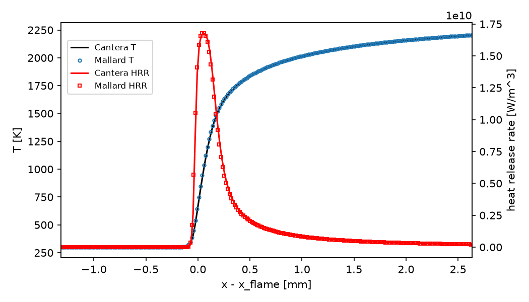
CH4/air with GRI-3.0 (53 species) costs about 15x more per step and needs 4-20x more steps per flame time (slower flames, the acoustic time step): 0.4-1.0 million steps for five flame times at 20 cells per delta_T. The sweep (tools/flame_sweep.py, examples/premixed_flame/ch4 for phi = 1) therefore runs on A100s, one 300-cell flame at 16.5 ms per step, or 5-8 flames sharing a GPU through MPS at 13-28 ms per step each. Every flame runs five flame times at CFL 1 (the time step of main); S_c and S_d are taken over the last flame time:

CH4/air, phi	0.6	0.8	1.0	1.2	1.4
Cantera S_L [m/s], mixture-averaged	0.1144	0.2711	0.3758	0.3325	0.1388
Mallard S_c error, 10 cells per delta_T	-2.42%	-2.50%	-3.08%	-4.19%	-3.53%
Mallard S_c error, 20 cells	-0.97%	-1.17%	-1.31%	-1.82%	-1.11%
Mallard S_c error, 40 cells	-0.37% (2.2 flame times)	-0.70% (3.4 flame times)	-0.78% (4.0 flame times)	-1.01% (3.4 flame times)	-0.60% (2.2 flame times)
Mallard S_d error, 20 cells	-1.12%	-1.48%	-1.62%	-2.08%	-1.38%
Cantera S_L [m/s], unity Lewis	0.1177	0.2460	0.2865	0.2132	0.1048
Mallard S_c error, 10 cells	-2.29%	-1.14%	-1.00%	-2.07%	-2.82%
Mallard S_c error, 20 cells	-0.69%	-0.45%	-0.42%	-0.72%	-0.80%
Mallard S_c error, 40 cells	-0.61% (4.1 flame times)	-0.40%	-0.30%	-0.35%	-0.32% (3.3 flame times)
Mallard S_d error, 20 cells	-0.77%	-0.79%	-0.82%	-1.05%	-0.94%

At 20 cells per delta_T every consumption speed is within the 2% criterion: mixture-averaged 1.0-1.8% slow, unity Lewis 0.4-0.8% slow; 10 cells is not enough (1.0-4.2% slow). At 40 cells the mixture-averaged errors roughly halve (0.4-1.0% slow; the runs marked with fewer than five flame times are still settling, slowly downward), while the unity-Lewis ones level off at 0.3-0.6% slow, like the H2 flames' offset. The displacement speeds are 0.1-0.4% below the consumption speeds (mixture-averaged phi = 1.2: 2.1% slow). The flames take about two flame times to relax from Cantera's discretization to Mallard's, longer than the H2 flames' half flame time, which is why the earlier 1.5-flame-time run at phi = 1 was still drifting; over the last two flame times the 20-cell consumption speeds vary by at most 0.4% (mixture-averaged phi = 1.2 by ±0.2% around its mean). Peak heat release is within 3.1% of Cantera's and the temperature within 6-19 K at 20 cells. CFL 0.5 against 1 (phi 0.6, 1.0 and 1.4, both models, at equal times over 2.5 flame times): the consumption speeds differ by at most 0.05%, against the 0.5% criterion.

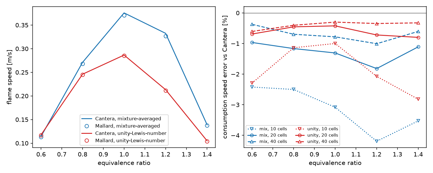
On a CPU core, chemistry is 68% of the H2 flame's step (h2o2) and 75% of the CH4 flame's (GRI-3.0); transport is most of the rest of the latter.

Thermal diffusion (Soret effect)

physics.soret = true (mixture-averaged transport only, as in Cantera, whose 1D flames accept it with the mixture-averaged and multicomponent models) adds the thermal diffusion fluxes -D^T_k grad T / T to the species fluxes, with Cantera's mixture-averaged thermal diffusion coefficients (Cantera 3.2, MixTransport::getThermalDiffCoeffs): the model of Chapman & Cowling as given by Zirwes & Kronenburg 2025,

D^T_k  = W_k W D_km sum_(j != k) (1.2 C*_kj - 1) / (D_kj (W_k + W_j)) (Y_k a_j - Y_j a_k),
a_k    = (15/4) (mu_k / W_k) / (1 + 1.065 sum_(j != k) X_j Phi_kj / X_k)    (0 where Y_k < 1e-20),
D^T_k <- D^T_k - Y_k sum_j D^T_j                                       (so that they sum to zero)

with D_km the mixture-averaged coefficients, Phi_kj Wilke's mixing operator, and C*_kj the reduced collision integral of Monchick & Mason at T* = k_B T / epsilon_kj, fitted, as Cantera does, by a polynomial of degree 8 in ln T* over the table rows bracketing the mechanism's T* range (with the fits in the reduced dipole moment for polar pairs). The model covers every species, not only the light ones: in lean H2/air flames H and H2 carry almost all of the effect (they diffuse toward hot gas, D^T < 0), and the normalization moves the balance to the abundant species.

• Fluxes. j_k = -rho D_km (W_k / W) grad X_k + Y_k V_c - D^T_k grad T / T. The thermal diffusion fluxes sum to zero, so the correction velocity stays that of the Fickian part, as in Cantera's 1D flames; the energy flux carries their enthalpy sum_k h_k j_k (without it, the temperature wave of the test below ends 2.7% off the conduction-only solution). D^T_k is computed per cell with the other coefficients and averaged to faces; grad T / T uses the face's T and gradient, as the heat flux. Walls, symmetry planes and outflow faces carry no thermal diffusion flux, as they carry no species flux. No Dufour effect (as Cantera).
• Time step. Unchanged: thermal diffusion couples the species to T one way and adds no diffusive eigenvalue.
• Cost. One more pass over the species pairs, with a degree-8 polynomial: on one A100 the properties alone go from 3.6 to 11.9 ns per cell for h2o2 (10 species, 1M cells) and from 172 to 424 ns for GRI-3.0; a step of the 2D lean H2 flame (examples/flame_2d, 72,576 cells, where chemistry is 90% of the step) from 20.5 to 22.3 ms (+9%).
• Off by default, and runs without it are bitwise identical to before (checked on CPU and GPU on premixed flames with both transport models).
• TFLES thickens D^T_k with the other molecular diffusivities; output DT_<species>.

Verification (test/chemistry_transport_test.cpp, test/mixture_transport_test.cpp, test/mpi_test.cpp): the coefficients match Cantera's at random states of h2o2 and GRI-3.0 (with absent species and a pure species) to 6e-13 of their largest magnitude and sum to zero; in an H2/N2 mixture at uniform composition and pressure with a temperature wave (600 +- 30 K, 1 mm), the hydrogen mode grows as the linear solution with Fickian relaxation, -D^T k^2 dT_0 / (rho T_0) (exp(-a k^2 t) - exp(-D_12 k^2 t)) / ((D_12 - a) k^2) (to 0.5%; zero without the option), while the temperature wave decays at lambda / (rho cp) (to 0.03%); runs are bitwise identical on 1 and 2+ ranks.

Validation against Cantera's FreeFlame with the same model (soret_enabled, mixture-averaged; tools/flame_reference.py --soret, examples/premixed_flame/reference/soret_flames.csv): the V8 setup above (20 cells per delta_T, CFL 0.2, two flame times, consumption speed over the last third), H2/air at 300 K and 1 atm:

H2/air, phi	0.4	0.5	0.6	1.0
Cantera S_L [m/s], mixture-averaged	0.16013	0.42969	0.80829	2.33237
Mallard S_c error	+0.40%	+0.19%	+0.28%	+0.21%
Cantera S_L [m/s], with Soret	0.15516	0.39969	0.73527	2.13546
Mallard S_c error	-0.58%	-0.07%	+0.34%	+0.41%
Mallard S_d error	-0.16%	-0.01%	+0.24%	+0.23%
Soret effect on S_L, Cantera	-3.10%	-6.98%	-9.04%	-8.44%
Soret effect on S_L, Mallard (S_c)	-4.05%	-7.23%	-8.98%	-8.26%
Peak Y_H with Soret, Mallard / Cantera	1.013	1.016	1.014	1.006

All within the 2% criterion; the Soret effect, 3-9% here, is reproduced to within a point (at phi = 0.4, the slowest flame, over two flame times, its two errors of +0.4% and -0.6% add up). Profiles aligned at the maximum of dT/dx differ from Cantera's by at most 0.3-1.5% of the peak for T and Y_H2 and 1.3-5% for H, O and OH at phi = 0.4-0.6, up to 3-9% at phi = 1, where the profiles are steepest (as without thermal diffusion, see above). Runs: 300 cells, OpenMP, 3 threads, 4.3-5.1 ms per step (thermal diffusion +11%), up to 1.3M steps at phi = 0.4.

Multicomponent transport: assessment

Cantera's multicomponent model (MultiTransport, the L-matrix formulation of Dixon-Lewis 1968) replaces the mixture-averaged diffusion coefficients by the full matrix D_kj, with fluxes j_k = rho (W_k / W^2) sum_j W_j D_kj grad X_j - D^T_k grad T / T, and also changes the conductivity and the thermal diffusion coefficients. Per state it assembles the 3K x 3K L matrix (A*, B*, C* collision integrals for every pair, Parker's rotational relaxation), solves it by LU for the conductivity and D^T_k, and inverts its K x K block for D_kj: O(9 K^3) work and O(10 K^2) memory per cell, against O(K^2) for the mixture-averaged model.

A device port of it (one cell per thread, local arrays, LU with partial pivoting; a prototype, not merged) matches Cantera's lambda, D_kj and D^T_k to 1e-14 for h2o2 and GRI-3.0. On one A100:

Properties per cell	mixture-averaged	with Soret	multicomponent
h2o2 (10 species), 1M cells	3.6 ns	11.9 ns	213 ns (59x, 18x)
GRI-3.0 (53 species), 20k cells	172 ns	424 ns	57,700 ns (336x, 136x)

The 2D lean H2 flame above costs 282 ns per cell and step; the multicomponent properties alone, at three RK stages, would add 640 ns (3.3x the step), before the O(K^2) fluxes per face and the K^2 matrix per cell they need (100 doubles for h2o2, 2,809 for GRI-3.0: 22 GB for a million cells). For GRI-3.0 one thread per cell also holds 300 KB of local arrays. What it buys, from Cantera's flames (soret_flames.csv): flame speeds within 0.1-3% of the mixture-averaged ones, and the same Soret effect to within a point:

H2/air, S_L [m/s]	phi 0.4	0.5	0.6	1.0
mixture-averaged	0.16013	0.42969	0.80829	2.33237
+ Soret	0.15516 (-3.1%)	0.39969 (-7.0%)	0.73527 (-9.0%)	2.13546 (-8.4%)
multicomponent	0.16520	0.43639	0.80862	2.28956
+ Soret	0.16095 (-2.6%)	0.40929 (-6.2%)	0.74458 (-7.9%)	2.11317 (-7.7%)

Decision: not now. Thermal diffusion is the larger effect (3-9% here) and the mixture-averaged model carries it at +9% of a flame's step; the multicomponent model's remaining 1-4% (1.1-1.3% at phi = 0.6-1, 3.6% at phi = 0.4, a weakly burning flame) would multiply the step cost by about four for hydrogen and is out of reach for larger mechanisms with one thread per cell. A later implementation should not port the L matrix as is: the iterative algorithms of Ern & Giovangigli (a few O(K^2) conjugate-gradient or Jacobi iterations from the mixture-averaged approximation, which converge to the exact coefficients; see Ern & Giovangigli 1998 for their thermal diffusion in H2 and CH4 flames) keep the mixture-averaged cost scaling, and the fluxes can use the matrix-vector product without storing D_kj.

Inviscid runs

type = "euler" with a mechanism means reactive Euler: species are advected and react, and no transport data is needed (species in the YAML without transport data are accepted). Numerical diffusion then sets the reaction-zone structure, which is the standard model for detonation studies; the validation suite measures resolution in points per half-reaction length.

7. Mechanism input

Format

Cantera YAML (format reference), read in C++ with yaml-cpp (MIT, FetchContent) at startup on every rank (mechanism files are small). Supported:

Feature	First	Later
ideal-gas phase, elements, species	yes
Thermo: NASA7, NASA9, constant-cp (the last for verification against the perfect-gas solver)	yes
Reactions: elementary (Arrhenius), three-body, explicit reverse rates, duplicate, non-integer orders	yes
Falloff: Lindemann, Troe, SRI	yes
pressure-dependent-Arrhenius (PLOG), Chebyshev		milestone 8
chemically-activated, Blowers-Masel, two-temperature-plasma, interface and electrochemical reactions		out of scope
Transport: gas model data (LJ, polarizability, rotational relaxation, dipole)	yes
Units (units: sections), phase selection by name	yes

Unsupported entries are errors that name the reaction, never silently dropped. Chemkin files are converted with Cantera's ck2yaml once, which also checks them.

TOML

[physics]
type = "navier_stokes"            # or "euler"
gas = "mixture"                   # "perfect" (default) keeps the gamma/R/mu inputs
mechanism = "mechanisms/h2o2.yaml"
phase = "ohmech"                  # optional; default: the first phase
transport = "mixture_averaged"    # "unity_lewis", "constant_lewis"; ignored for euler
lewis = { H2 = 0.3, H = 0.18 }    # constant_lewis; others default to 1

[chemistry]
enabled = true                    # false: non-reacting multicomponent flow
integrator = "rosenbrock"         # later "bdf", "rkc"
coupling = "strang"               # later "sdc"
rtol = 1.0e-6
atol = 1.0e-10
T_frozen = 0.0                    # no chemistry below this T
load_balance = true               # MPI: redistribute chemistry cost (section 4)

[initialize]
type = "constant"
u = [0.0, 0.0]
p = 101325.0
T = 300.0
X = { H2 = 2.0, O2 = 1.0, AR = 7.0 }     # or Y = {...}; normalized; unlisted species are 0

# analytical: one expression per listed species, plus "balance" for the rest
# Y = { H2 = "x < 0.5 ? 0.028 : 0.0", O2 = "x < 0.5 ? 0.226 : 0.233" }
# balance = "N2"

[[boundaries]]
zone = "left"
type = "upt"
u = [10.0, 0.0]
p = 101325.0
T = 300.0
X = { CH4 = 1.0, O2 = 2.0, N2 = 7.52 }

X/Y are accepted wherever a boundary or initial state takes T. A [chemistry] table without gas = "mixture" is an error.

8. Boundary conditions

Every boundary keeps its meaning; the exterior state gains Y and the surrogate (gamma, e0):

Boundary	Species	Thermo
extrapolation, image faces	from the image	from the image
symmetry, walls	interior Y (zero normal diffusive flux)	interior (wall temperatures and heat fluxes enter the diffusive fluxes only)
upt, farfield, dirichlet	given Y/X (expressions for dirichlet)	from given p, T, Y
p_out, p_out_average	interior Y	interior gamma

farfield uses the Riemann invariants with each side's frozen gamma. Catalytic walls and species-specific wall fluxes are out of scope.

Milestone 3 supports extrapolation, symmetry, wall_adiabatic (slip for euler, no-slip for navier_stokes from milestone 9), upt and p_out for mixtures; farfield, dirichlet and p_out_average are rejected at input until they are needed. The composition of upt may vary along the boundary (stratified inflows such as a mixing layer feeding a triple flame): each value of X or Y can be an expression in x, y, z, with an optional balance species as in [initialize]. Each face then gets its own copy of the condition, with the composition, density and surrogates at its center, so the flux kernels are unchanged.

9. Output and restart

• VTU variables: Y_<name>, X_<name> (any species, or Y_*, X_* for all), T, HRR (heat release rate -sum_k h_k W_k omega_k), OMEGA_<name>, MW, GAMMA, CP, CHEM_COST (sub-steps in the last step), and with transport MU, LAMBDA, D_<name>.
• Restart format version 2: the header gains the list of variable names, so restarts map fields by name: RHO, RHOU_*, RHOE, then RHOY_<species>, then the auxiliary fields T_SEED (the cached Newton seed of T, named apart from the output variable T, which is recomputed from the state) and CHEM_H (last chemistry sub-step). The auxiliary fields make restarted runs bit-identical (they seed Newton and the chemistry step size). Reading checks the species names against the mechanism; a restart can start a reacting run from a non-reacting multicomponent one, and a mechanism change that keeps names (e.g. a reduced mechanism) maps by name, with missing species set to zero after an explicit allow_missing_species = true. Version 1 files still read for perfect-gas runs.
• Diagnostics: check_interval prints min/max T, max |sum Y - 1|, the number of active chemistry cells and the max/mean sub-steps, and the chemistry wall time fraction.
• 0D tool: MallardReactor, a small executable built from the same kernels, runs constant-volume or constant-pressure reactors from TOML and writes CSV. It backs the 0D validation and the chemistry benchmarks without a mesh.

10. Milestones

Each is a reviewable PR with its tests; nothing reacting is user-visible until milestone 8 (the 0D tool arrives in milestone 7).

1. State split. State {flow, species} with zero species everywhere: time integrators, axpby, halo exchange, restart v2 with names. Bit-identical results; restart v1 still read. (Species conservation sums come with the first species, in milestone 3.)
2. Mechanism and thermo. yaml-cpp, Cantera YAML reader (species, NASA-7/9, units), device thermo tables, T from e. Tests against Cantera tables (generated by a Python script in tools/, committed as small CSV files).
3. Non-reacting mixtures, first order and MUSCL. Gas-model template on the RHS kernels, Riemann solvers on (W, gamma, e0) (Rusanov, HLL, HLLC), species fluxes, shared-limiter MUSCL, X/Y in initial and boundary conditions, VTU species output, species conservation sums. Tests: constant-cp single-species mixture reproduces the perfect-gas solver; species interface advection; multicomponent shock tube.
4. TENO for mixtures. Primitive characteristic reconstruction of the flow block, shared-stencil scalars, theta bounds, W-based troubled indicator. Tests: design order on smooth species advection; interface and shock tube tests at TENO5.
5. Double flux (input option). Tests: interface advection keeps p, u uniform to round-off; shock tube energy error reported.
6. Kinetics. Rate tables, elementary/three-body/falloff, production rates and analytical Jacobian. Tests: rates vs Cantera at random states; Jacobian vs finite differences.
7. 0D reactor and integrator. Rosenbrock with dense LU; MallardReactor. Tests: ignition delays and equilibrium end states vs Cantera.
8. Coupling. Strang splitting in the solver; [chemistry] input; active-cell queue; PLOG and Chebyshev. Tests: reactive shock tube, 1D detonation (CJ speed, ZND structure).
9. Transport. Species fits, mixture-averaged, unity and constant Lewis, diffusion fluxes with correction velocity, enthalpy diffusion, viscous time step. Tests: properties vs Cantera; premixed flame speed.
10. GPU performance. Team-per-cell kernels, layout study, cost binning, sparse LU for large mechanisms, benchmark suite with recorded baselines.
11. MPI. Chemistry load balancing; chemistry cost in partition weights. Tests: rank-count independence with chemistry; imbalance benchmark. Done: state migration (chemistry.load_balance), the slowest rank's chemistry time in the summary, and the measurements of section 5; partition weights not added.
12. Extensions, each optional and driven by need: Roe/RHLL for mixtures (done); BDF integrator; SDC coupling; mechanism-specialized (code-generated) kernels; 2D cellular detonation, counterflow flame and mixing-layer cases.

11. Validation suite

Three tiers, all automated:

• Unit (GoogleTest, every PR, seconds): exact or round-off criteria.
• Verification (GoogleTest, every PR, under a minute on CPU): small runs with reference data in test/data/.
• Validation and benchmarks (validation/, run per milestone and before releases, CPU and A100): full cases with scripts that produce the comparison plots and a pass/fail table.

Reference data from Cantera is produced by Python scripts in tools/ with the mechanism file used by the run, and committed as small CSV files with the Cantera version recorded, so the tests themselves need no Cantera. Same mechanism, same thermo and transport, so differences are Mallard's numerics.

Mechanisms used throughout: the H2/O2 submechanism of GRI-Mech 3.0 with Ar and N2 (mechanisms/h2o2.yaml, 10 species, 29 reactions, from Cantera's data; it stands in for Burke et al. 2012, whose file Cantera does not ship, and can be swapped for it without code changes), GRI-Mech 3.0 (53 species, 325 reactions; source, ships with Cantera), and for performance a ~100-species skeletal mechanism (e.g. HyChem Jet-A, Wang et al. 2018) and a detailed ~500-1000-species mechanism (LLNL n-heptane, Curran et al. 1998, or iso-octane, Curran et al. 2002). Species counts are taken from the files when they are added.

Unit and verification tests

Test	Reference	Pass criterion
YAML reader	Cantera's parsed values	Every coefficient of the three mechanisms equal to Cantera's after unit conversion (relative 1e-14)
Thermo: cp, h, s, g per species and mixture, T(e)	Cantera at 200 random (T, Y)	Relative 1e-12 (double), 1e-5 (float); T(e(T)) within 1e-10 K
Production rates and rates of progress, every reaction type	Cantera net_production_rates at 1000 random (T, p, Y)	Relative 1e-10 where |omega| > 1e-12 max |omega|
Analytical Jacobian	Centered finite differences of our rates	Relative 1e-6 per entry (scaled by row norm)
Transport fits and mixture properties	Cantera mixture-averaged	Relative 1e-6
Perfect-gas regression	Current solver	All existing tests bit-identical without a mechanism
Single-species constant-cp mixture	Perfect-gas solver, same gamma, R	Sod and 2D Riemann: agreement to 1e-12 (different arithmetic, same scheme)
sum Y = 1, positivity, conservation	Exact	max |sum_k rho Y_k - rho| / rho < 1e-13 (1e-5 float) after 1000 steps of a multispecies Riemann problem; min Y_k >= 0; each sum_cells V rho Y_k conserved to round-off without chemistry
Species advection, smooth	Exact (translated profile)	Design order of MUSCL and TENO3-5 on triangles, quads, tets, hexes
Rank and thread independence	Single rank, one thread	Reacting 2D case on 1-4 ranks and 1/4 threads: bit-identical
Restart	Uninterrupted run	Reacting case restarted mid-run: bit-identical

Validation cases

#	Case	Reference	Pass criterion	Milestone
V1	0D constant-volume ignition delay, H2/air (Burke) and CH4/air (GRI-3.0), T0 1000-1500 K, phi 0.5-2, 1 and 10 atm (MallardReactor and a single-cell solver run)	Cantera IdealGasReactor at tight tolerances	Ignition delay (max dT/dt) within 0.5%; T(t) and major species within 1% over the trajectory	7
V2	Equilibrium end states of V1	Cantera equilibrate("UV")	T within 0.1 K, major species within 1e-4 absolute	7
V3	Large-mechanism ignition (~100 and ~500+ species)	Cantera	As V1; also the performance baseline	7, 10
V4	Species interface advection, 1D and 2D (skewed triangles), H2 or He into air at different T, uniform p and u	Exact: uniform p, u	Conservative scheme: report max |p - p0| / p0 and require it to converge under refinement; double flux: p, u uniform to 1e-12 after 10 flow-throughs	3, 5
V5	Thermally perfect multicomponent shock tube (non-reacting, Fedkiw, Merriman & Osher 1997 type, H2/O2/Ar)	Exact Riemann solution for the thermally perfect mixture (our own iterative solver in tools/, Cantera thermo)	L1 errors of rho, u, p, T, Y converge at the expected rate (about 1 for discontinuous data); no overshoot of Y	3, 4
V6	Reactive shock tube: H2:O2:Ar = 2:1:7, reflected-shock ignition turning into a detonation (Fedkiw et al. 1997; Martinez Ferrer et al. 2014 for the viscous version and a resolution study)	Converged Mallard run and published profiles at 170 and 230 us	Detonation front within 2 cells of the converged position; peak T and p converge under refinement	8
V7	1D CJ detonation, 2H2-O2-7Ar at 6.67 kPa and H2/air, driven by an overdriven start	CJ speed and ZND profile from the Shock and Detonation Toolbox (Cantera-based, same mechanism)	Mean front speed within 1% of D_CJ at 20+ cells per half-reaction length; ZND induction length within 5% and von Neumann state approached under refinement	8
V8	Premixed laminar flame speed, H2/air and CH4/air at phi = 0.6-1.4, 1 atm, mixture-averaged and unity Lewis	Cantera FreeFlame (same transport model)	Flame speed within 2% at 20+ cells per thermal thickness; difference between CFL 0.2 and 0.1 below 0.5% (splitting error); temperature and HRR profiles overlaid	9
V9	2D cellular detonation, 2H2-O2-7Ar at 6.67 kPa	Oran et al. 1998, Gamezo, Desbordes & Oran 1999, Deiterding's AMROC results; experimental cell widths	Regular cells; cell width within published numerical range at matched resolution; soot-foil (max p) image	12
V10	Counterflow diffusion flame, H2/N2 vs air, strain-rate sweep	Cantera CounterflowDiffusionFlame	Peak T vs strain within 2% near the axis, accepting that a 2D/3D opposed-jet run only approximates the similarity solution	12
V11	Shock/H2-bubble interaction with detailed transport, or a reacting mixing layer	Billet, Giovangigli & de Gassowski 2008	Code-to-code: interface and shock positions; grid convergence	12

V10 (examples/counterflow_diffusion, tools/counterflow_reference.py, counterflow_setup.py, plot_counterflow.py): H2/N2 (1:3) against air at 300 K and 1 atm, nozzles 10 mm apart, momentum-balanced, against Cantera's CounterflowDiffusionFlame swept in strain up to extinction. Cantera's is the axisymmetric similarity solution, which has no exact planar equivalent; the case predates Mallard's axisymmetric formulation (axisymmetric.md), so the run is 3D: a quarter of two opposed round plug jets (r < 5 mm) with N2 coflows, symmetry planes and side pressure outlets, 15 cells per FWHM of the temperature profile along the axis, started from Cantera's solution. Strain is measured on the stagnation line in both, as the local strain rate of the oxidizer stream K_ox (the first maximum of -du/dx ahead of the flame) and as the spread rate V_T = v / r at the peak temperature. From U_o = 1 to 4.6 m/s (K_ox 344-1640 1/s, up to 90% of Cantera's extinction strain rate of 1816 1/s) the steady peak temperature is within 2% of Cantera's at the same K_ox (+0.41% to +1.96%), so V10 passes, but the excess grows with strain and is mostly not a resolution error (at 4 m/s it is the same at 10 and 15 cells per FWHM; at 2 m/s it falls from 0.74% to 0.34% between 10 and 22). The finite jets give the flame less strain for the same K_ox than the similarity solution (V_T / K_ox 0.89 against 0.95 at 4 m/s), by an amount that depends on the jets: with 7.5 mm jets the excess at 4 m/s reaches 1.9% and was still rising. At matched V_T the peak temperatures agree within 0.3-0.6% everywhere on the branch, for both jet widths, and 1.0% at Cantera's extinction strain. Mallard's flame still burns at K_ox = 1818 1/s (U_o = 5.1 m/s) and goes out at 5.6 m/s (K_ox 1890-1975 1/s while burning), so its extinction strain rate is 0-9% above Cantera's. Stagnation-line temperature, velocity and species profiles overlay Cantera's at matched K_ox. Results, plots and the resolution and domain-size variants are in the example's README.

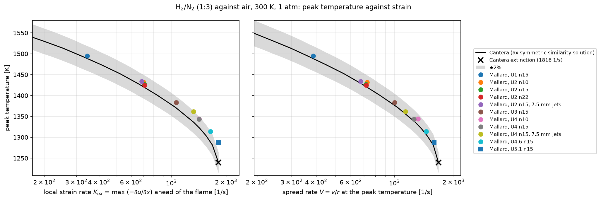
Flame-wall interaction (tools/flame_wall.py): head-on quenching of the stoichiometric H2/air flame (h2o2.yaml, mixture-averaged transport, 300 K, 1 atm; Cantera: S_L = 2.332 m/s, T_b = 2379 K, thermal thickness delta_T = 329 um, delta_L = lambda_u / (rho_u cp_u S_L) = 19.9 um) against an isothermal wall at 300 K. A 1D strip of 4 um cells, started from Cantera's flame 0.4 mm from the wall with the fresh gas at rest and the burnt gas leaving through a pressure outlet; MUSCL, HLLC, SSPRK3, CFL 1. The wall heat flux is the solver's (the boundary cell's conduction to the wall), the flame position the wall distance of the largest H2 consumption rate. The flame quenches at x_q = 90 um, with a peak wall heat flux of 2.19 MW/m^2: Pe_q = x_q / delta_L = 4.5 (x_q / delta_T = 0.27) and phi_q = q_max / (rho_u cp_u S_L (T_b - T_u)) = 0.38. Classical head-on quenching gives phi_q 0.34-0.4 and Pe_q near 3 for hydrocarbon flames (Vosen, Greif & Westbrook 1984; Poinsot, Haworth & Bruneaux 1993); hydrogen's delta_L is several times smaller for a quenching distance similar to heptane's (Owston, Magi & Abraham 2007), so its Pe_q is larger. Conduction across the quenching distance, int_Tw^Tb lambda dT / x_q (Cantera's burnt-gas conductivity), predicts phi_q = 0.45, consistent with the measured 0.38 (the gas next to the wall is cooler than T_b at quenching). With 2 um cells: x_q = 89 um, 2.22 MW/m^2, phi_q = 0.39 (within 1% of the 4 um run). Runs: 256k steps in 17 min (4 um) and 907k in 62 min (2 um) on one A100, chemistry 90%.

Performance benchmarks

• Chemistry throughput: cells advanced per second per A100 (and per CPU node) for one splitting step of dt = 1e-8 s (detonation regime) and 1e-6 s (flame regime), on states sampled from V1/V3 trajectories (mix of fresh, igniting and burnt), versus species count (Burke 13, GRI 53, ~100, ~500+). Reported with the sub-step histogram and against Cantera/CVODE on one CPU core, and against the published GPU numbers of Niemeyer & Sung 2014, Curtis et al. 2017 and Balos et al. 2024 where the mechanisms match.
• Imbalance: the same with 1% of cells igniting, which measures the team-per-cell and binning strategies.
• Full solver: time per cell-step and the chemistry/flow split for V7 and V8 in 2D and 3D; multi-GPU weak scaling of V9 with and without chemistry load balancing.
• Baselines are recorded per milestone; a regression above 10% blocks a PR touching the chemistry kernels.

Risks

Risk	Mitigation
Chemistry dominates run time on large mechanisms and our integrator is slower than mature libraries	Benchmarks against published throughput from milestone 7; the integrator interface lets a BDF or codegen path, or a library backend, replace Rosenbrock without touching the solver
Conservative scheme gives unacceptable pressure oscillations for injection-type problems	Species-interface test quantifies it from milestone 3; double flux is designed in and scheduled
Shared-stencil species reconstruction is too dissipative for thin radical layers	TENO smooth cells already use the high-order central stencil; measured by the flame and ZND tests; per-species stencil selection can be added for selected species
Strang splitting error in steady flames	Two-CFL flame test; SDC-style forcing designed into the integrator interface
GPU register pressure in rate kernels for large mechanisms	Team-per-cell with scratch memory; reactions grouped by type; codegen path as a later option
Static partitions become badly imbalanced at fronts	Chemistry-state load balancing (no mesh change), then dynamic rebalancing per mpi.md
Float builds produce wrong chemistry	Chemistry in double always; float validated on non-reacting cases and on 0D tests only
Porting Cantera's transport fitting is subtle	Property tests to 1e-6 against Cantera; unity_lewis works without it

Decisions on the open questions

Accepted by the user (2026-10-02):

1. Detonations first (milestone 8 before transport in milestone 9).
2. Own chemistry core (~3-5k lines) rather than waiting for a Kokkos 5 TChem.
3. Dependencies: yaml-cpp via FetchContent; Cantera (Python) only for generating committed reference data in tools/.
4. Double flux as a non-conservative input option; conservative by default.
5. HLLC first; Roe/RHLL for mixtures stay in milestone 12 (since done).
6. Chemistry always in double, also in float builds.
7. Scope of "done": as in milestone 12, the 2D cellular detonation and counterflow flame are extensions, not requirements for the first reacting release.