Documentation of the main branch

These pages follow Mallard's main branch, which is ahead of release 0.8.0: some features they describe come with the next release.

Supersonic flow over a cone

A sharp cone of 15° half-angle in a Mach 2 stream at zero incidence carries an attached conical shock. Between the shock and the cone the inviscid flow depends only on the angle θ from the axis, and the ordinary differential equation of Taylor and Maccoll (1933) gives it exactly. This tutorial meshes the flow with tetrahedra in Gmsh, runs Mallard's 3D Euler solver on a CPU, a GPU or several MPI ranks, and checks the shock angle and the surface pressure against that solution.

You will use: a Gmsh mesh with named boundary zones, symmetry planes, a supersonic inflow, a characteristic far field and an outflow, line probes, surface output and wall forces. Files: tutorials/cone/. Setup: Tutorials.

1. Geometry

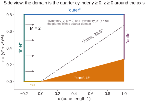
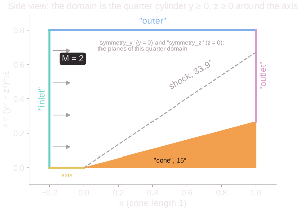
The cone has its tip at the origin, its axis along x and unit length. The flow is symmetric about the axis, so a quarter of it is enough: the domain is the quarter cylinder y ≥ 0, z ≥ 0 of radius 0.8 around the axis, from 0.2 upstream of the tip to the cone's base, with symmetry planes at y = 0 and z = 0. Its outer surface stays clear of the shock, which leaves the base at r = tan 33.9° = 0.67.

The exact solution comes from taylor_maccoll.py:

mkdir -p run/cone && cd run/cone
python3 $MALLARD/tutorials/cone/taylor_maccoll.py --mach 2 --cone 15

M = 2.0, cone 15.0 deg: shock angle 33.9147 deg, surface p/p_inf 1.56629, Cp 0.20225, Mach 1.7069

It integrates the equation inward from the state behind an oblique shock of trial angle β until the angular velocity vanishes, which marks the cone's surface, and finds the β whose surface angle is 15°. It also writes the solution between cone and shock, taylor_maccoll.csv.

2. Mesh

cone.geo builds the domain with Gmsh's OpenCASCADE kernel (a cylinder minus the cone, intersected with the box y, z ≥ 0), names the six boundary zones as physical surfaces, and sets the cell size with a background field: h within 40° of the axis, where the shock lies, h_out outside.

cp $MALLARD/tutorials/cone/input.toml .
gmsh $MALLARD/tutorials/cone/cone.geo -3 -o cone.msh                       # h = 0.02: 100,000 tetrahedra
gmsh $MALLARD/tutorials/cone/cone.geo -3 -setnumber h 0.01 -o cone.msh    # 728,000 tetrahedra

Mallard reads each physical surface as a boundary zone of the same name, which [[boundaries]] refers to; a boundary face in no physical group would form the zone unassigned, which the input would then have to assign too.

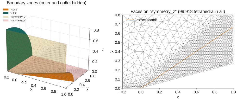
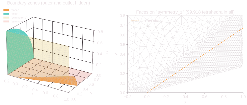
python3 $MALLARD/tutorials/cone/plot_mesh.py cone.msh --out . draws these two figures from the mesh file.

3. Input file

input.toml works in units of the free stream: density and sound speed 1, so the velocity is the Mach number, 2, and p = T = 1/γ with a gas constant of 1 (p_ref = T_ref = 1/γ, rho_ref = 1).

Table	In this case
[run]	t_stop = 3, five passes of the flow over the cone, at CFL 1
[mesh]	type = "file", cone.msh
[initialize]	The free stream everywhere (type = "constant")
[[boundaries]]	cone: wall (wall_adiabatic, a slip wall for the Euler equations); inlet: upt, the free stream imposed (all characteristics enter); outer: farfield; outlet: extrapolation (all leave); symmetry_y, symmetry_z: symmetry
[numerics]	HLLC, SSPRK3, MUSCL with the Venkatakrishnan limiter
[physics]	euler, γ = 1.4
[[forces]]	The force on the cone, every 10 steps, forces_cone.csv
[[probes]]	40 points across the shock layer at x = 0.8 in the plane y = z, every 20 steps, probe_layer.csv
[[write_data]]	Every 0.5: the volume (solut/flow), the cone's faces (geometry = "cone") and the symmetry plane z = 0 (geometry = "symmetry_z") with the values of their cells

4. Run

On a CPU with 8 threads (6,500 steps; minutes for h = 0.02):

$MALLARD/build-3d/src/Mallard -i input.toml --kokkos-num-threads=8

On several MPI ranks, which split the mesh between them (results are the same bit for bit):

mpirun -n 4 $MALLARD/build-3d/src/Mallard -i input.toml

On a GPU, with a CUDA build of the 3D solver (-DMallard_DIM=3, see the first simulation), the same input runs unchanged: h = 0.02 takes under 2 minutes on one A100, h = 0.01 (13,800 steps) about 10.

5. Monitor

Every 100 steps Mallard prints a progress row: step, time, time step, fraction done, wall time per step, throughput, time left, and the minimum density, minimum pressure and maximum Mach number. Here the maximum Mach number stays at 2.0 (the free stream) and the minimum pressure at about p∞ = 0.714; a NaN or a negative pressure stops the run (check_nan).

The probes and forces are written as the run goes, so they can be plotted at any time. plot_results.py (next section) draws them over time: the pressure at two probe points, one inside the shock layer and one just outside the shock, and the cone's pressure drag coefficient, (F_x − p∞ A) / (q∞ A) with A the base area of the quarter cone, which for a cone of uniform surface pressure equals the surface Cp.

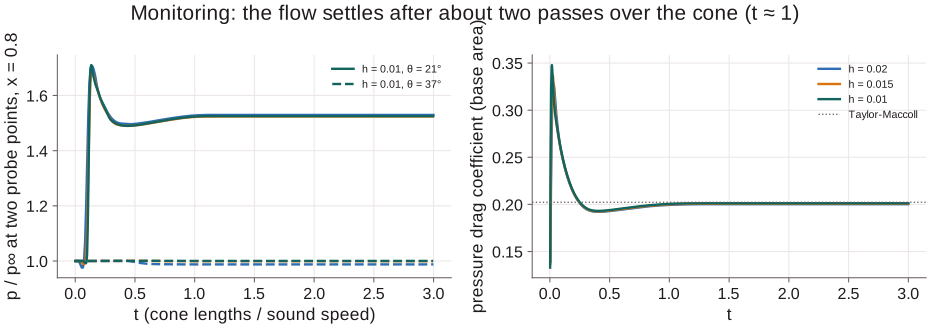
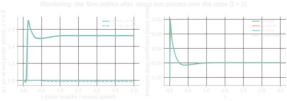
The flow is steady after about two passes over the cone, t ≈ 1; the run goes on to t = 3 to be sure.

6. Post-process and compare

python3 $MALLARD/tutorials/cone/plot_results.py . --out .

reads the last snapshot of each output series (solut/*.pvd) and the probe and force files, prints the measured shock angle (where the probe line crosses halfway up the exact pressure jump) and the surface pressure coefficient averaged over 0.3 ≤ x ≤ 0.95, and draws the figures of this page. With several runs, e.g. one directory per mesh, it compares them: plot_results.py h020 h015 h010 --labels "h = 0.02" "h = 0.015" "h = 0.01".

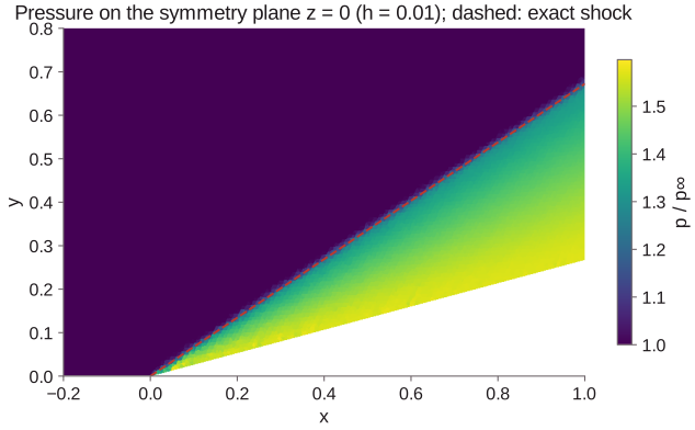
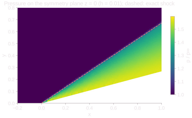
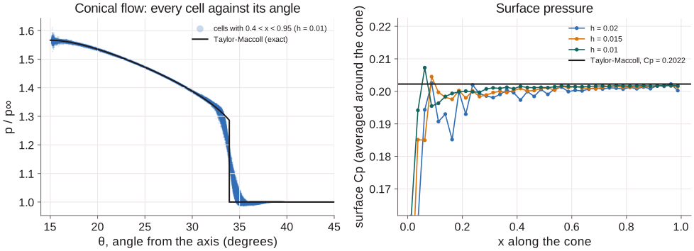
The pressure rises across the shock and then isentropically toward the cone. Since the flow is conical, every cell of the volume, plotted against its angle θ = atan(r / x), should fall on the one curve of the exact solution:

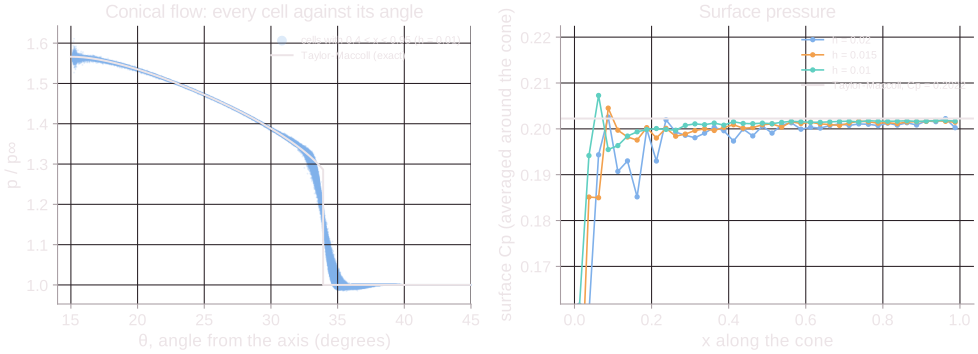
Mesh	Tetrahedra	Shock angle	Surface Cp (0.3 ≤ x ≤ 0.95)
h = 0.02	100,000	34.12° (+0.20°)	0.2005 (−0.85%)
h = 0.015	225,000	33.70° (−0.21°)	0.2011 (−0.57%)
h = 0.01	728,000	34.08° (+0.16°)	0.2015 (−0.36%)
Taylor-Maccoll		33.91°	0.2022

The cells collapse onto the exact curve; the shock is spread over two to three cells, centered on the exact angle. Near the tip the cone is thinner than a cell and the surface pressure is low; from x = 0.3 on, it is within a fraction of a percent of the exact value.

7. Things to try

• Higher order. Replace MUSCL by TENO-E (type = "TENO", order = 3, with bound_preserving = true at the shock) and compare the shock width.
• Another cone or Mach number. -setnumber cone_angle 20 in Gmsh and --cone 20 for the exact solution; check that the shock still clears the outer boundary (R), and change u of [initialize], inlet and outer for another Mach number.
• Detached shock. Above about 40° at Mach 2 no conical solution exists (taylor_maccoll.py finds no shock angle); the shock stands off the tip and the flow is no longer conical.