Documentation of the main branch
These pages follow Mallard's main branch, which is ahead of release 0.8.0: some features they describe come with the next release.
Examples
Run each case from its own directory, e.g.
cd examples/riemann_2d
../../build/src/Mallard -i input.toml --kokkos-num-threads=8
python ../../tools/animate.py solut riemann
Shocks and compressible flow
sod
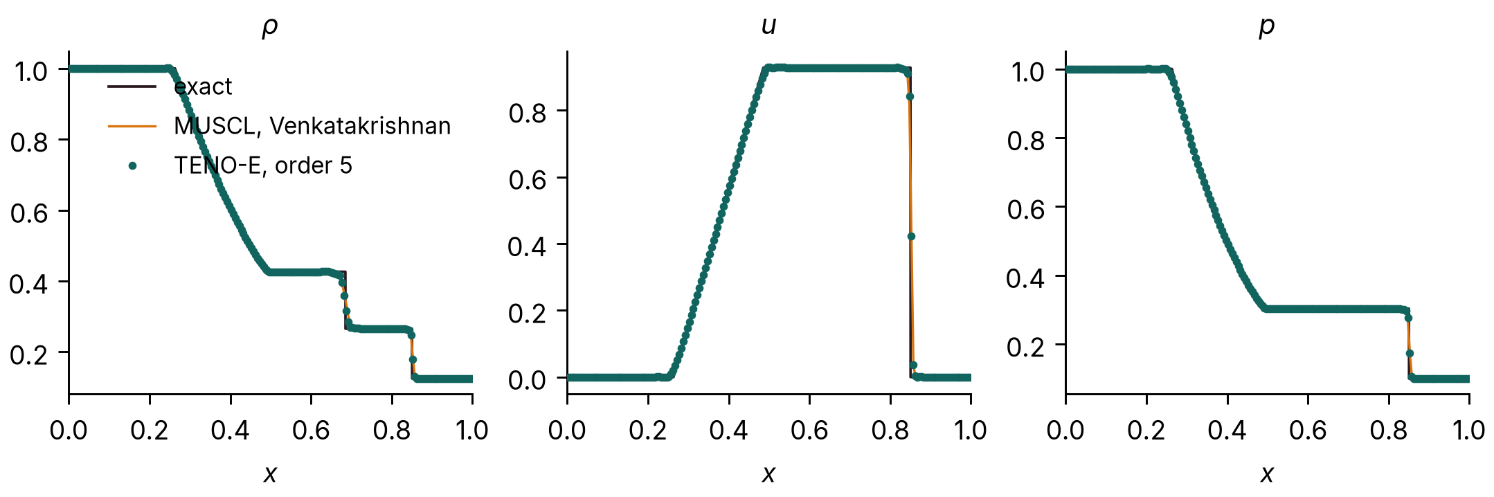
Sod shock tube with TENO5 on a 200x4 strip
Size, time on 12 CPU threads: 800 cells, seconds. Input file · results
shu_osher
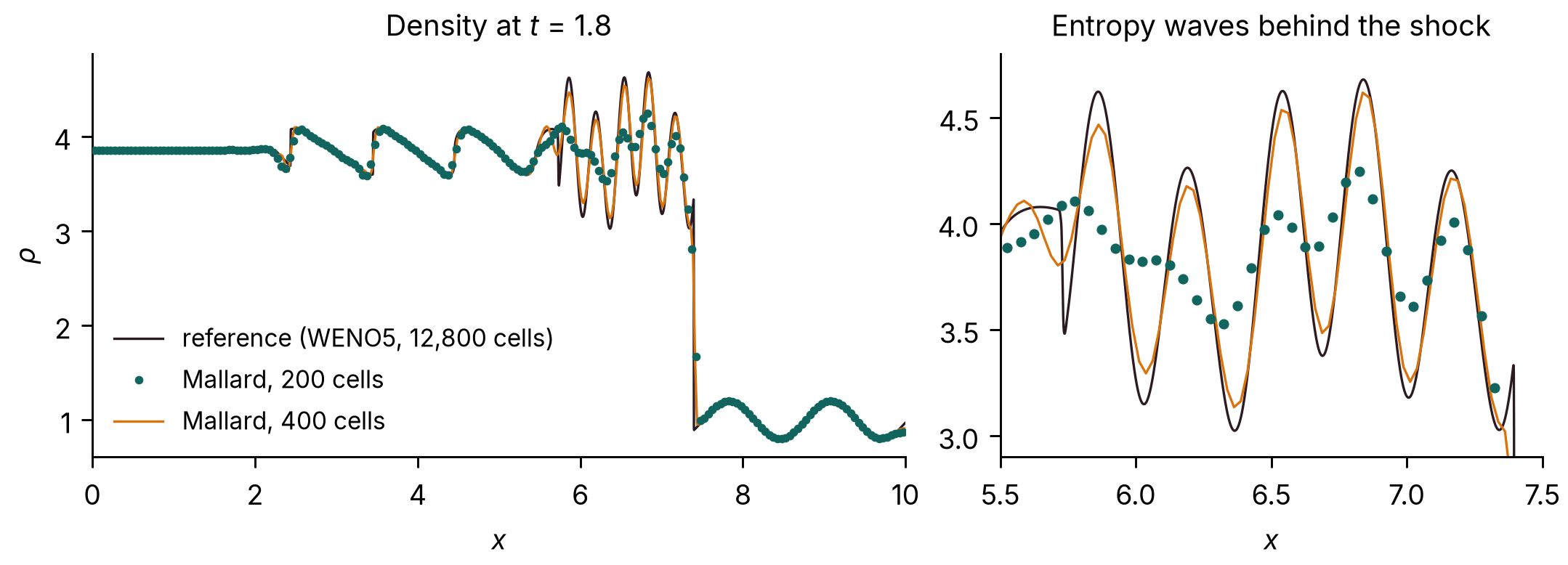
Mach 3 shock running into an entropy wave, the standard test for high-order schemes
Size, time on 12 CPU threads: 800 cells, seconds. Input file · results
riemann_2d
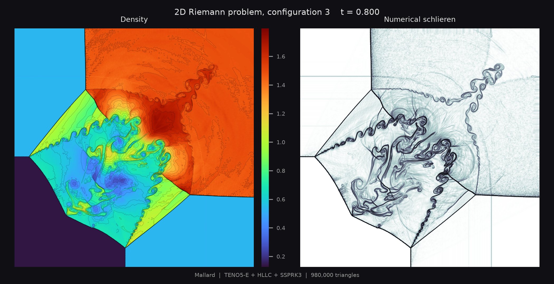
2D Riemann problem, configuration 3, on 320,000 triangles with TENO5
Size, time on 12 CPU threads: ~20 minutes. Input file · results
riemann_2d_quads
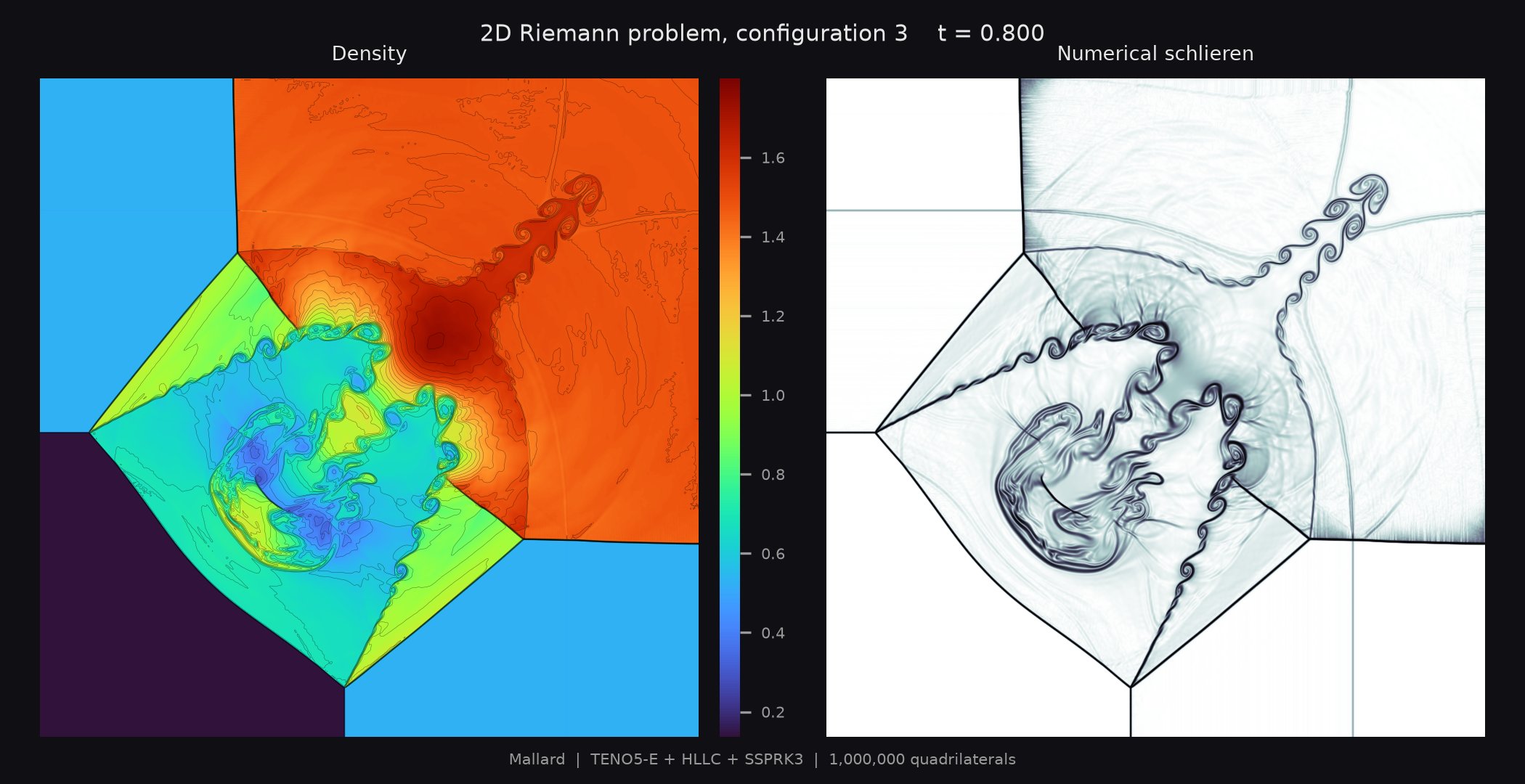
The same problem on 160,000 quadrilaterals
Size, time on 12 CPU threads: ~9 minutes on 6 threads. Input file · results
double_mach
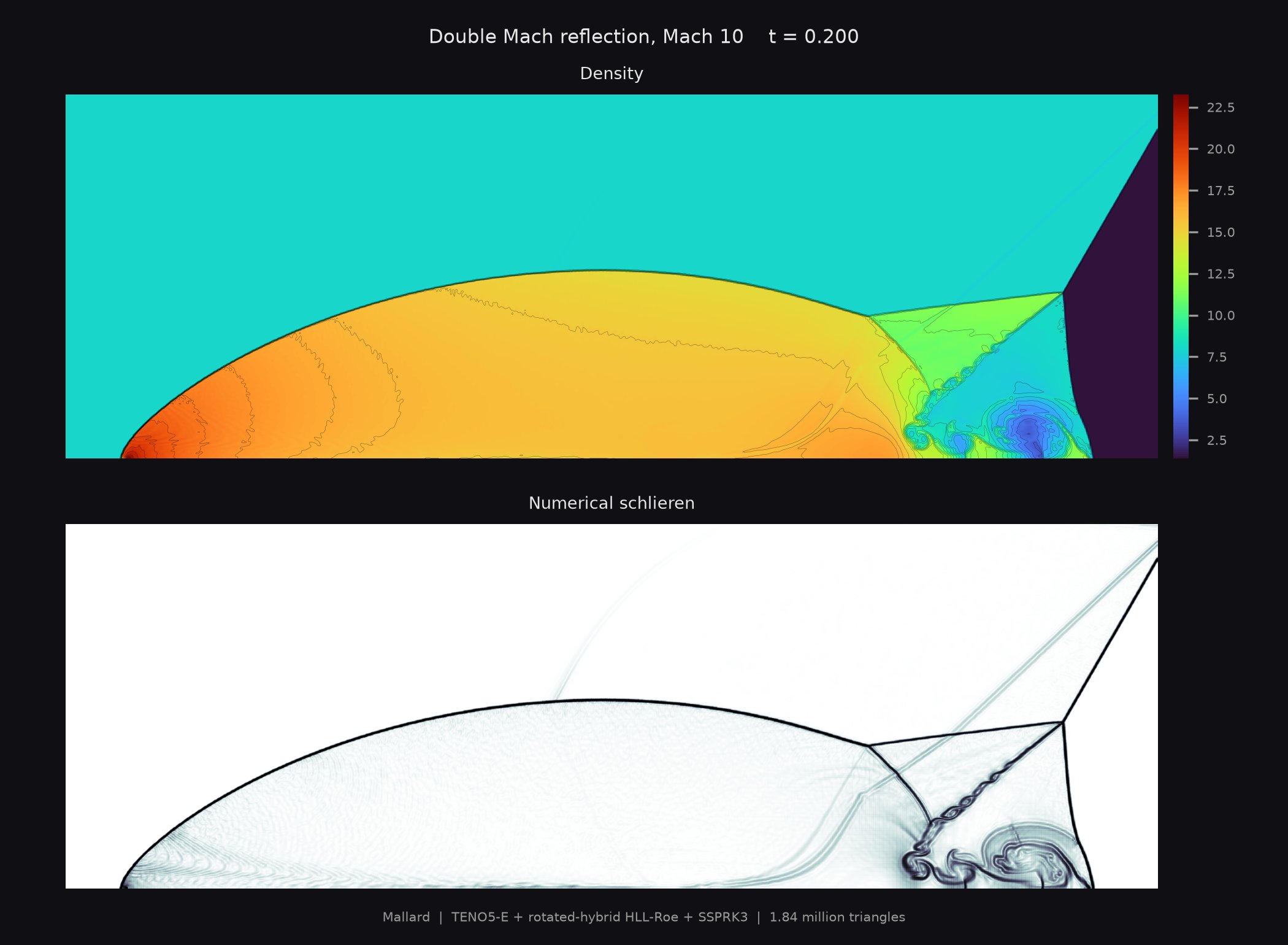
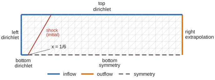
Double Mach reflection of a Mach 10 shock: a split bottom boundary (inflow, then wall) and an exact moving shock on the top boundary
Size, time on 12 CPU threads: 460,000 triangles, ~1 hour. Input file · results
wedge
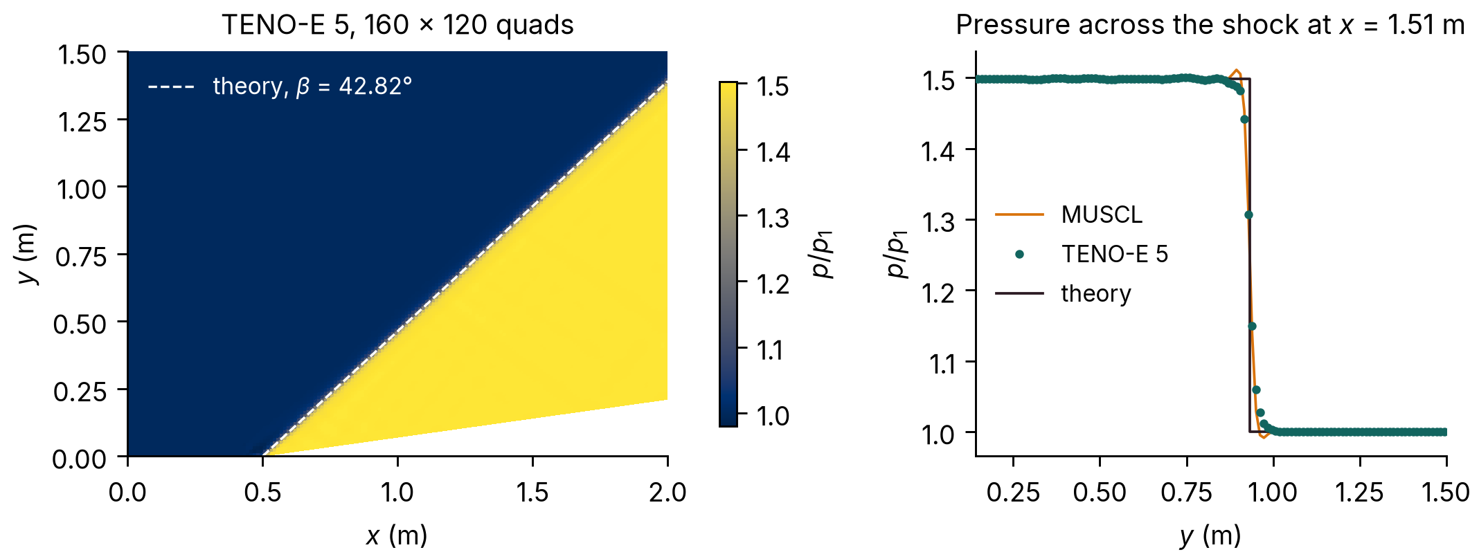
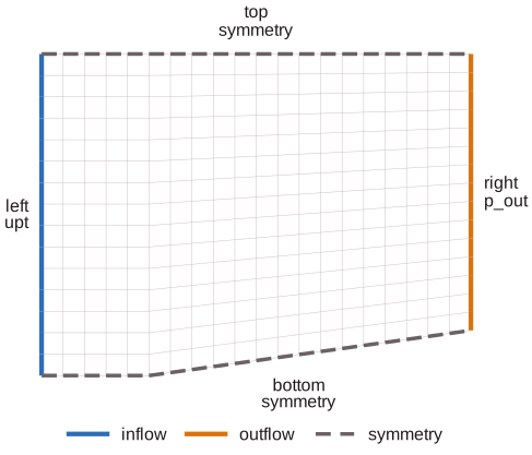
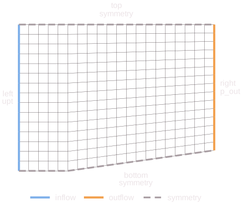
Mach 1.76 flow over an 8 degree ramp; the oblique shock matches theory (p2/p1 = 1.498)
Size, time on 12 CPU threads: 19,200 quads, minutes. Input file · results
explosion_3d
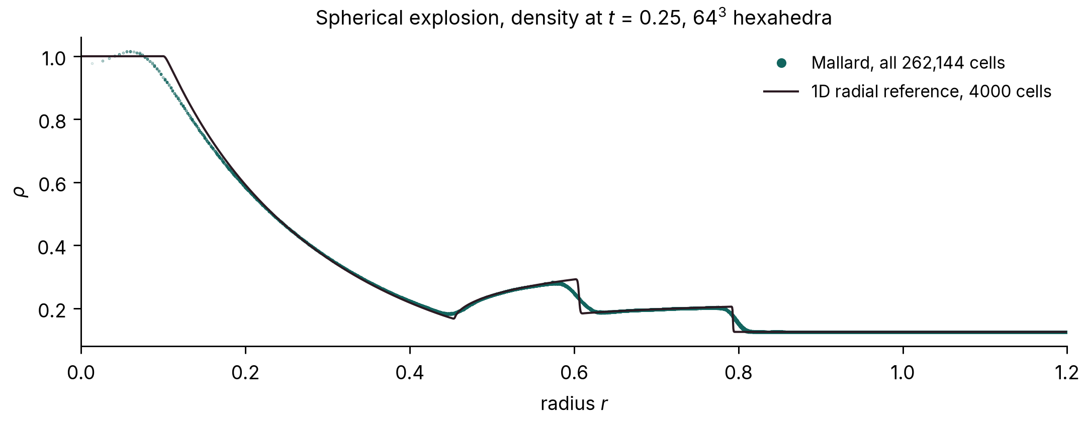
Spherical explosion (3D build): one octant with symmetry planes, TENO5 on 64^3 hexahedra; the solution stays spherically symmetric
Size, time on 12 CPU threads: 262,144 cells, ~5 minutes on 8 threads. Input file · results
sedov_3d
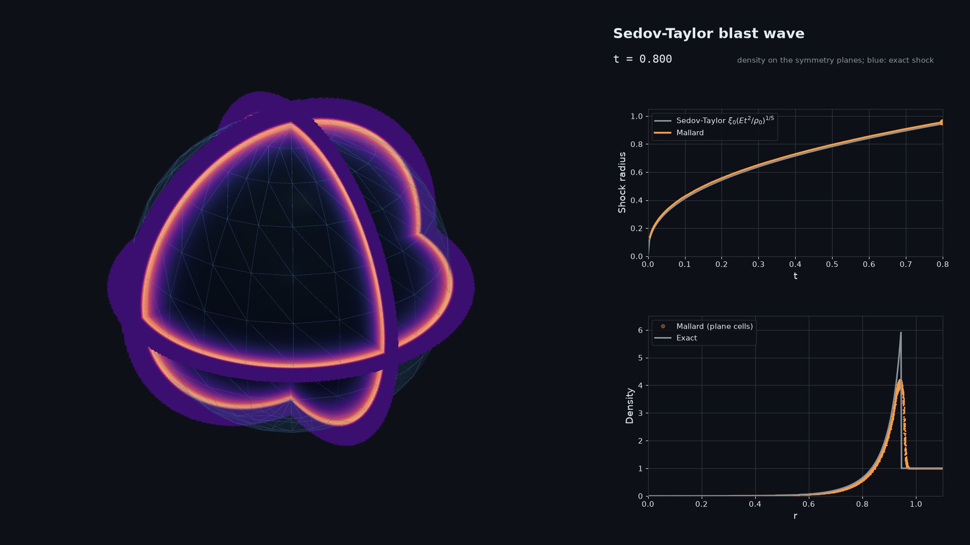
Sedov-Taylor point blast (3D build): one octant, bound-preserving TENO5 on 128^3 hexahedra, against the exact similarity solution (tools/sedov.py). The shock radius stays within 1-3% of R = 1.0328 (E t^2 / rho0)^(1/5)
Size, time on 12 CPU threads: 2.1M cells, ~1.5 hours on four A100s. Input file · results
sphere_mach3
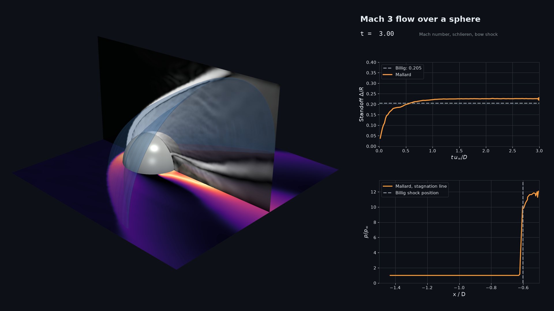
Mach 3 flow over a sphere (3D build) on an unstructured Gmsh tetrahedral mesh of the quarter domain (generate it with tools/make_sphere_mesh.py): HLL with bound-preserving TENO5. The bow-shock standoff settles at Delta / R = 0.226, 10% above Billig's correlation (0.205): 0.01 D, under half the tetrahedron edge length (0.025 D) in the shock layer
Size, time on 12 CPU threads: 800,000 tetrahedra, ~1.5 hours on four A100s. Input file · results
mallard
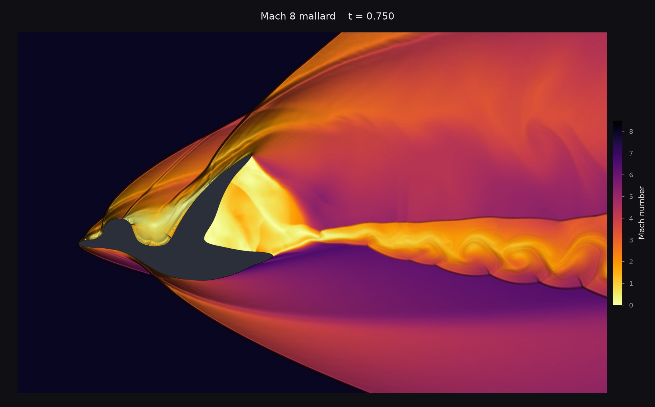
Mach 8 flow over a flying mallard from an impulsive start: RHLL with bound-preserving TENO5 on a Gmsh triangle mesh; generate the mesh with tools/make_mallard_mesh.py first
Size, time on 12 CPU threads: 1.07M triangles, ~1.5 hours on a GPU. Input file · results
Axisymmetric flows
poiseuille_pipe
Hagen-Poiseuille flow in a round pipe (axisymmetric), driven by a body force from rest: the steady profile converges to the exact one at second order (mean error 3.2e-4 U on 32 cells across the radius)
Size, time on 12 CPU threads: 128 quads, 1 minute on one thread. Input file
noh_axisymmetric
Spherical Noh implosion on the meridian plane (axisymmetric, bound-preserving TENO5): shock radius within 1% of t / 3 in every direction, post-shock density 62-63 of the exact 64 (higher in the first cells along the axis, the usual overshoot at symmetry lines)
Size, time on 12 CPU threads: 40,000 quads, ~2 minutes on 4 threads. Input file
sedov_axisymmetric
Sedov-Taylor blast as an axisymmetric run, against the exact solution (tools/sedov.py): shock radius 0.6% ahead of R(t) at t = 0.8, spherical to 2% at the density peak
Size, time on 12 CPU threads: 65,536 quads, 5 minutes on one A100. Input file
sphere_axisymmetric
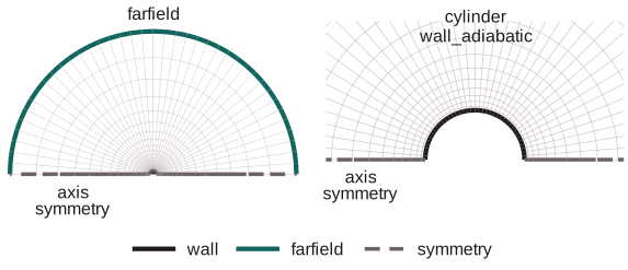
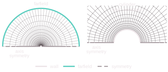
Steady flow past a sphere at Re = 100 and 150 (axisymmetric, Mach 0.2) on a half O-grid from tools/make_cylinder_mesh.py --half: drag within 1.2% of the Clift-Grace-Weber correlation, separation angle within 0.2 degrees, wake length 0.885 D and 1.21 D (Johnson & Patel: 0.88, about 1.2); check with tools/plot_sphere_axisymmetric.py
Size, time on 12 CPU threads: 16,384 quads, 285,000 viscous-limited steps: ~30 minutes on one A100. Input file
Viscous flows
viscous_shock_tube
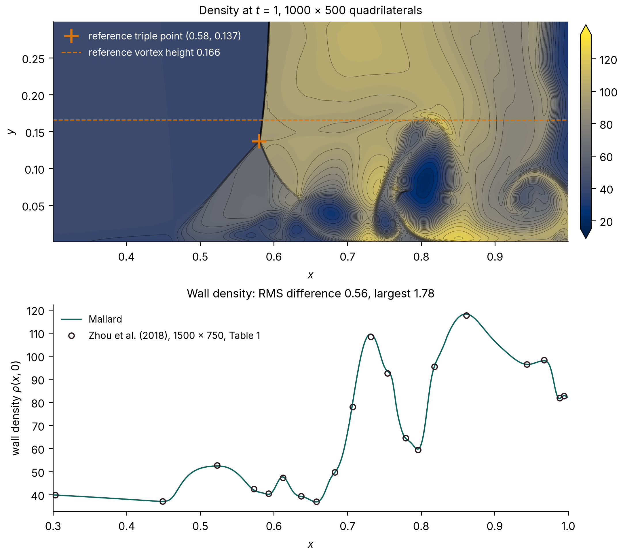
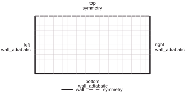
Daru & Tenaud viscous shock tube at Re = 200: shock / boundary-layer interaction in a closed box, giving a lambda shock and a primary vortex by t = 1. Matches the grid-converged wall density of Zhou et al. to 0.5 RMS; check with tools/plot_viscous_shock_tube.py
Size, time on 12 CPU threads: 500,000 quads, 58,500 viscous-limited steps: use a GPU build (or Nx = 500, Ny = 250: ~20 min on 6 threads). Input file · results
cylinder
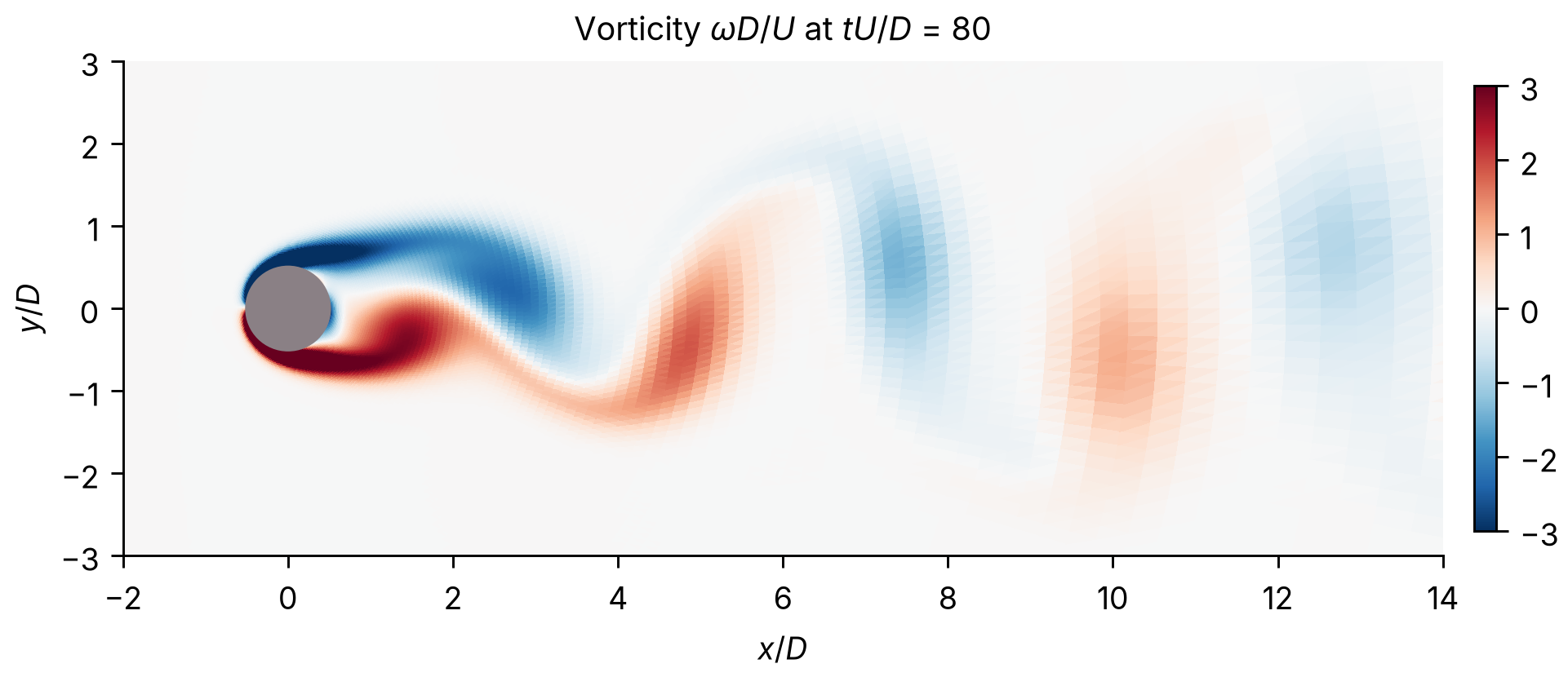
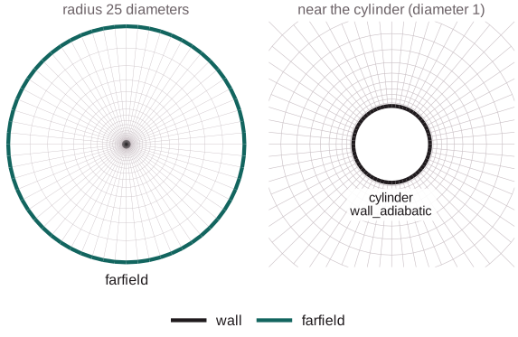
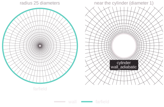
Viscous flow past a cylinder at Re = 100 (vortex shedding) on a Gmsh O-grid; generate the mesh with tools/make_cylinder_mesh.py first. Reproduces St, Cd and lift amplitude to within 2%
Size, time on 12 CPU threads: 49,152 quads, ~50 min on a laptop CPU. Input file · results
sphere_re300
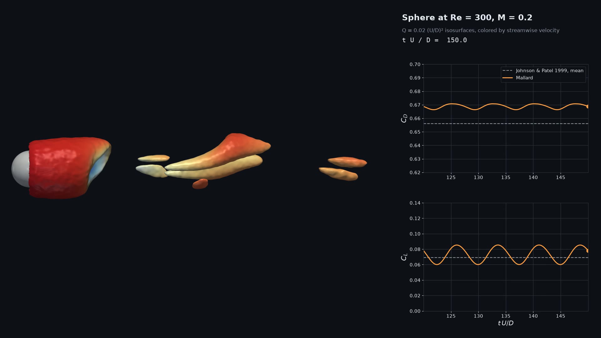
Viscous flow past a sphere at Re = 300 (3D build): periodic shedding of hairpin vortices, on a Gmsh mesh of prisms (boundary layer) and tetrahedra from tools/make_sphere_re300_mesh.py; MUSCL. St = 0.133, Cd = 0.669, Cl = 0.073 against 0.137, 0.656, 0.069 (Johnson & Patel 1999), within 0.2%, 0.4% and 5% of a mesh with 2.4 times the cells
Size, time on 12 CPU threads: 850,000 cells, 1.04M steps: ~4.7 hours on four A100s. Input file · results
Turbulence
taylor_green_3d
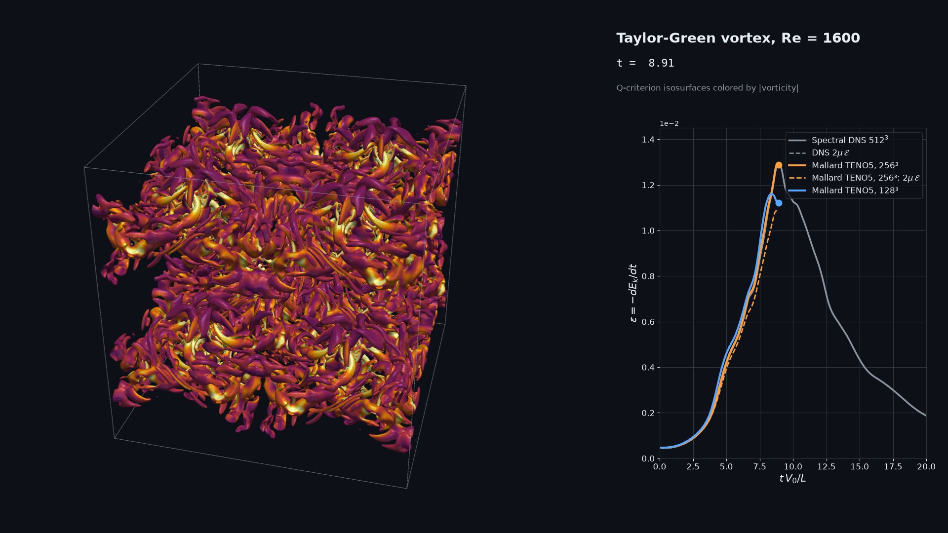
Taylor-Green vortex at Re = 1600 (3D build): the high-order workshop DNS case on the octant [0, pi]^3 with symmetry planes. At 64^3 per octant (128^3 full box) the dissipation peak is 0.01302 at t = 8.1, against 0.01286 at t = 9.0 for the 512^3 spectral DNS
Size, time on 12 CPU threads: 262,144 cells, 32,000 steps: ~1 hour on one A100. Input file · results
taylor_green_3d (input_periodic.toml)
The same case on the full periodic box [0, 2 pi]^3 (no symmetry planes), for runs on several GPUs
Size, time on 12 CPU threads: 128^3 = 2.1M cells. Input file
isotropic_turbulence
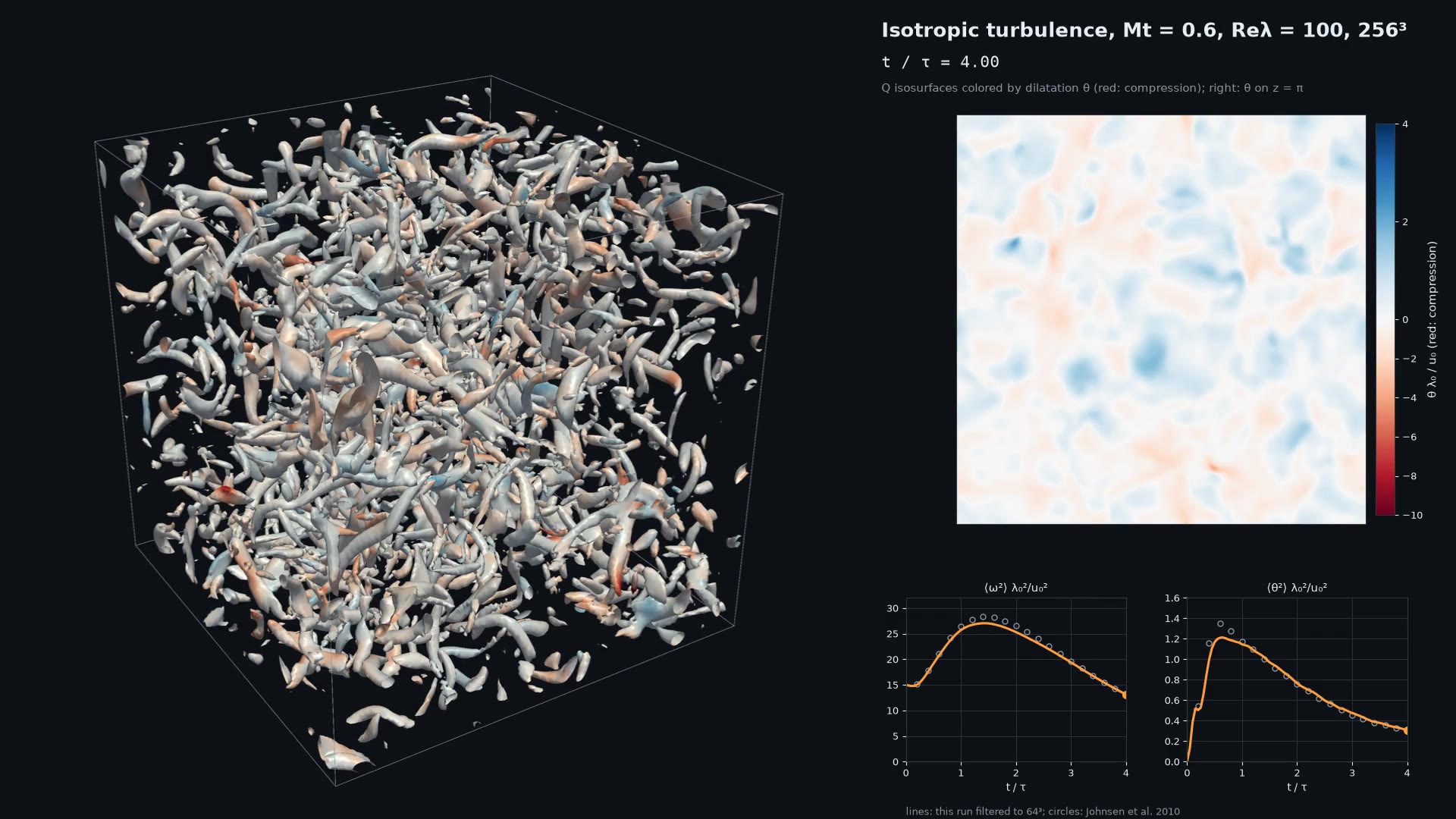
Decaying compressible isotropic turbulence with eddy shocklets (3D build), the case of Johnsen et al. (2010): Mt = 0.6, Re_lambda = 100, k0 = 4 on the periodic box, as DNS on 64^3, 128^3 and 256^3 hexahedra (TENO5) from the same random initial field (tools/isotropic_turbulence_restart.py). At 256^3 (k_max eta >= 2.7) kinetic energy, temperature and density variances are grid-converged to 0.3% and the enstrophy to 3%; filtered to 64^3 as the references, the enstrophy is within 2.4% (mean) of Johnsen et al.'s filtered 256^3 and 0.3% of Subramaniam et al.'s filtered 512^3, the dilatation variance within 0.6%. tools/isotropic_turbulence_stats.py, plot_isotropic_turbulence.py and animate_isotropic_turbulence.py analyze and animate it; details in the input's header
Size, time on 12 CPU threads: 16.8M cells, 4,307 steps: about an hour on 12 A100s (128^3: 17 minutes on 3). Input file · results
channel_retau180
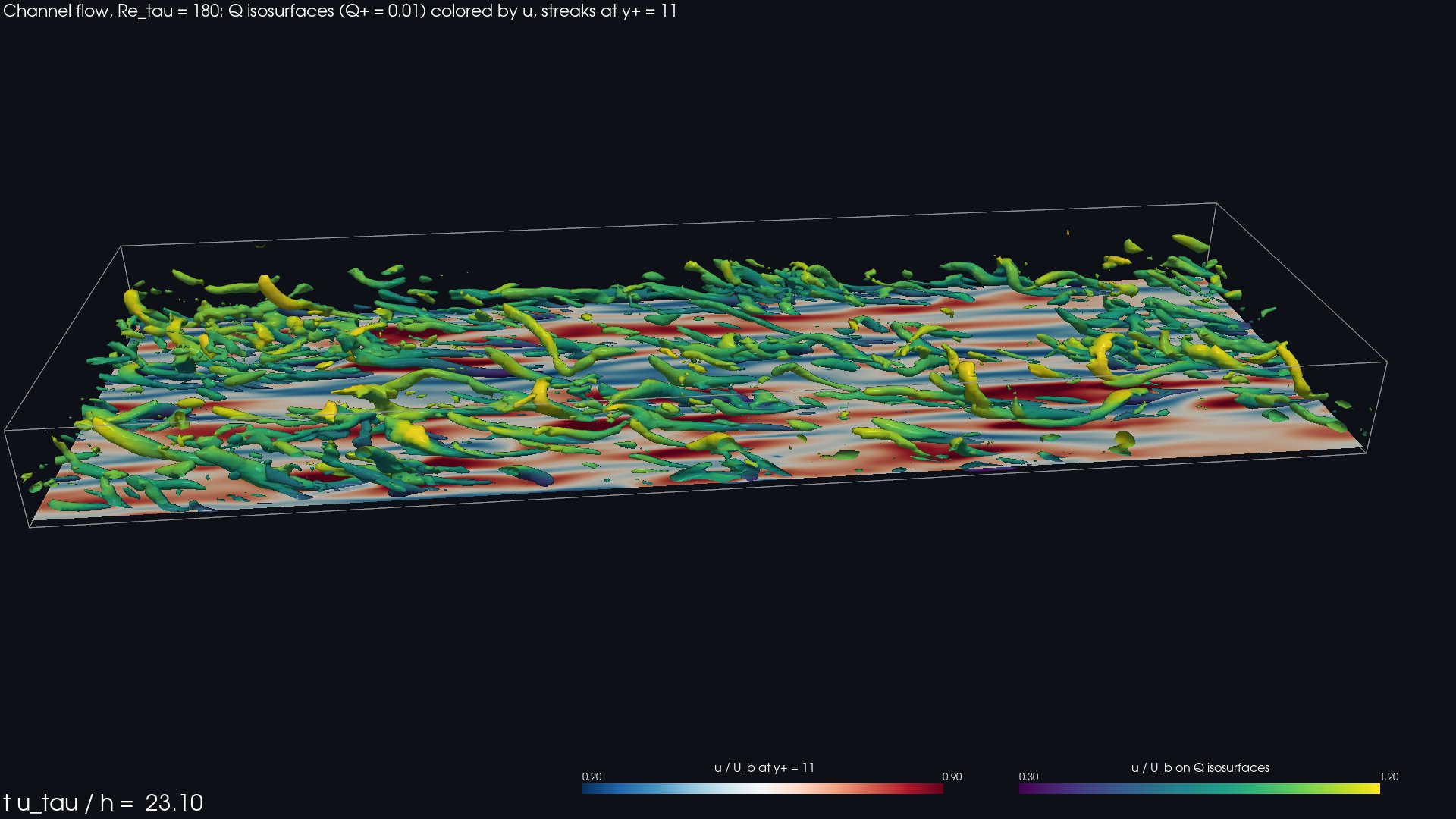
Turbulent channel flow at Re_tau = 180 (3D build): DNS at bulk Mach 0.2 between isothermal walls, periodic in x and z, on the 4 pi h x 2h x 4/3 pi h box of Moser, Kim & Mansour (1999), with the mass flow held by [source] mass_flow and a tanh-stretched generated mesh ([mesh] stretching); MUSCL with the kinetic-energy-preserving hybrid convective flux, and the kinetic-energy budget of [integrals] (numerical dissipation 0.9% of the total). Generate the initial state with tools/channel_init.py; [statistics], tools/plane_average.py and tools/plot_channel.py compare the profiles with MKM, tools/animate_channel.py animates the near-wall vortices. Over 12.9 h/u_tau: Re_tau = 180.8 against 178.1 (Cf 2.0% high), the RMS velocity and -u'v' peaks within 2%. The input's header lists the alternatives: HLLC at every face gives Cf 7% low on this mesh (its upwind dissipation is 7% of the total) and reaches MKM only on a mesh twice as fine in x and z
Size, time on 12 CPU threads: 2.36M cells (dx+ = 11.8, dz+ = 5.9, dy+ = 0.88 at the wall), 489,000 steps: 2.3 hours on two A100s. Input file · results
channel_inflow_retau180
Spatially developing turbulent channel at Re_tau = 180 (3D build): DNS with digital-filter synthetic turbulence at an nscbc_inlet, its mean profile and Reynolds stresses taken from the periodic channel_retau180 statistics (inflow_profile.csv). Wall shear, -u'v' and the RMS peaks recover to within 5% of the periodic channel by about 17h (Keating et al. 2004: about 20h); the outlet uses beta = 0 behind a sponge. Start from the periodic example's restart with tools/tile_restart.py (see the input's header)
Size, time on 12 CPU threads: 4.7M cells, 337,000 steps: 2.5 hours on four A100s. Input file
turbulent_inflow_duct
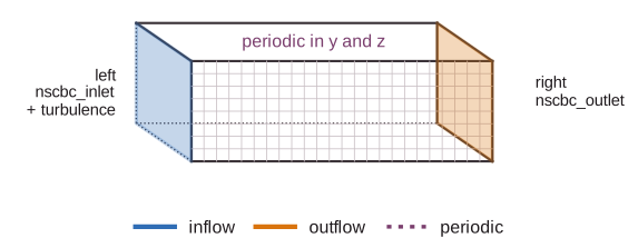
Isotropic digital-filter turbulence (u' = 0.1 U, L = 0.25, Re_L = 100) entering a duct periodic across and decaying downstream (3D build): inlet Reynolds stresses within 6% of target, and zero_net_flux removing the plane acoustic wave (spurious p'_rms 7.8 rho u'^2 without it, 1.1 by x = 20L with it)
Size, time on 12 CPU threads: 6.3M cells, 65,000 steps: 1.5 hours on one A100. Input file
Large-eddy simulation
cbc_les
Large-eddy simulation of decaying grid turbulence (Comte-Bellot & Corrsin 1971; 3D build) with the Sigma model and the hybrid KEEP/HLLC flux on 32^3 to 128^3 hexahedra (tools/cbc_les.py): spectra within 0.06-0.09 decades RMS of the measurements at 128^3 (and at 64^3 with C = 1.8), with 1-2% of the dissipation numerical; model off, the energy piles up at the grid cutoff; with HLLC alone, 84% of the dissipation is numerical. Details in the input's header and docs/design/les.md
Size, time on 12 CPU threads: 262,144 cells, 2,035 steps: 3 minutes on 4 CPU threads. Input file
channel_les
Wall-resolved LES of turbulent channel flow at Re_tau = 395 (3D build) against Moser, Kim & Mansour (1999): Sigma model with Scotti's filter width, hybrid KEEP/HLLC flux, 64^3 hexahedra. Re_tau within 0.7% (2.6% with Delta = V^(1/3)) against 7.1% without the model; mean velocity within 3% for y+ = 30-300; 3-5% of the dissipation numerical. Details in the input's header and docs/design/les.md
Size, time on 12 CPU threads: 262,144 cells, 857,000 steps: 65 minutes on one A100. Input file
channel_les (input_590.toml)
The same LES at Re_tau = 590 (96^3): Re_tau within 1.6% of MKM with the Sigma model (Scotti's width), 4.1% with V^(1/3), 7.8% without a model; 3% of the dissipation numerical. Details in the input's header and docs/design/les.md
Size, time on 12 CPU threads: 884,736 cells, about 900,000 steps: 3.5 hours on one A100. Input file
volvo_bluff_body
LES of the Volvo bluff-body combustor (Sjunnesson et al.; 3D build), non-reacting (cold.toml): Sigma, hybrid flux, digital-filter inflow and NSCBC outlet on a Gmsh hexahedral mesh from tools/make_volvo_mesh.py. Recirculation length 1.34 D against 1.35 D measured, RMS axial velocity within 0.08 U_b and mean within 0.14 U_b (0.08 downstream of x/D = 3.75) at the five LDA stations; eps_num / eps_sgs = -0.38. reacting.toml (propane-air with mechanisms/c3h8_2step.yaml, TFLES) is set up but not validated: details in the headers and docs/design/les.md, section 8.3
Size, time on 12 CPU threads: 2.7M cells, 626,000 steps: 2.8 hours on four A100s. Input files
flame_turbulence
Premixed H2/air flame in decaying turbulence (3D build): DNS reference (input.toml, 224 x 128 x 128, u' = 2.1 S_L, Ka = 2) and its LES with the thickened flame model (les.toml, Delta = 0.8 delta_L, F = 4): turbulent flame speed within 6-9% of the DNS with the default dynamic efficiency, and within 8-14% at Delta = 1.6 delta_L, where Colin's efficiency (efficiency = "charlette") doubles it. Details in the headers and docs/design/les.md, section 8.3
Size, time on 12 CPU threads: DNS 3.7M cells, 67,000 steps: 6-8 hours on 3-4 A100s; LES 15,360 cells, 7,044 steps: under a minute on one A100. Input file
Reacting flows and mixtures
h2_ignition
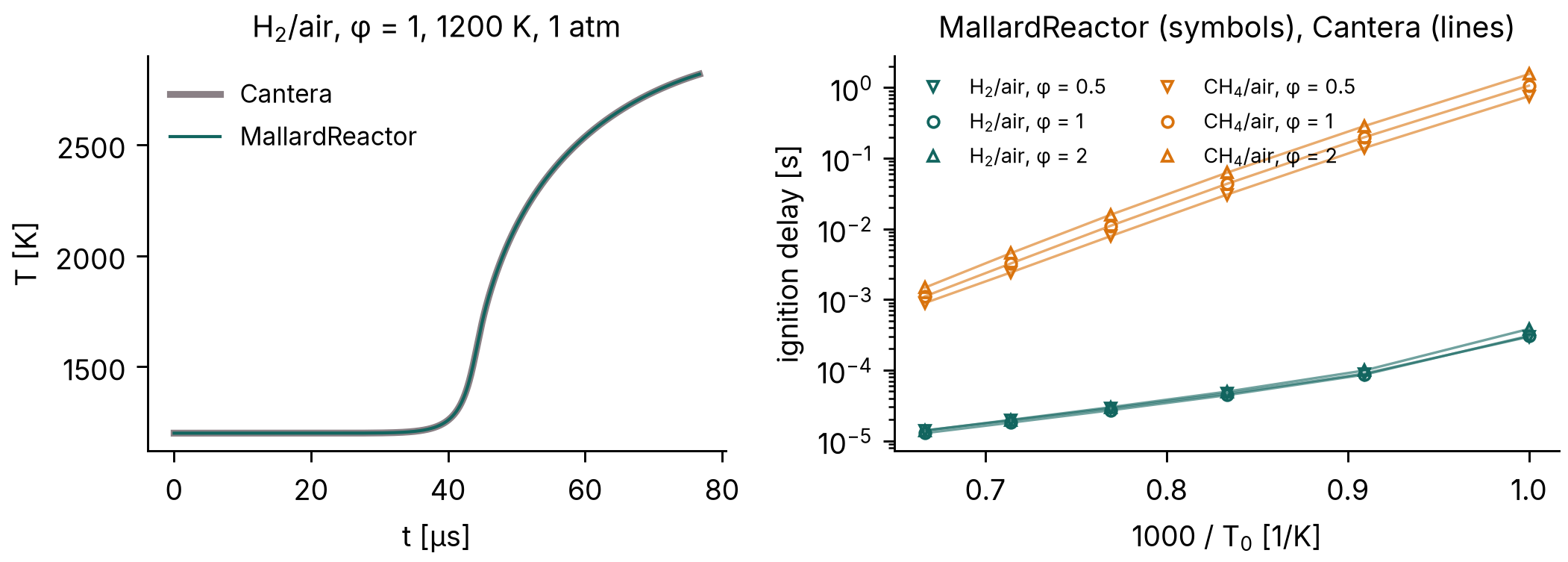
Constant-volume ignition of stoichiometric H2/air at 1200 K, 1 atm with MallardReactor (../../build/src/MallardReactor -i input.toml, writes reactor.csv); ignition delay 44.2 us as Cantera
Size, time on 12 CPU threads: 0D, milliseconds. Input file · results
reactive_shock_tube
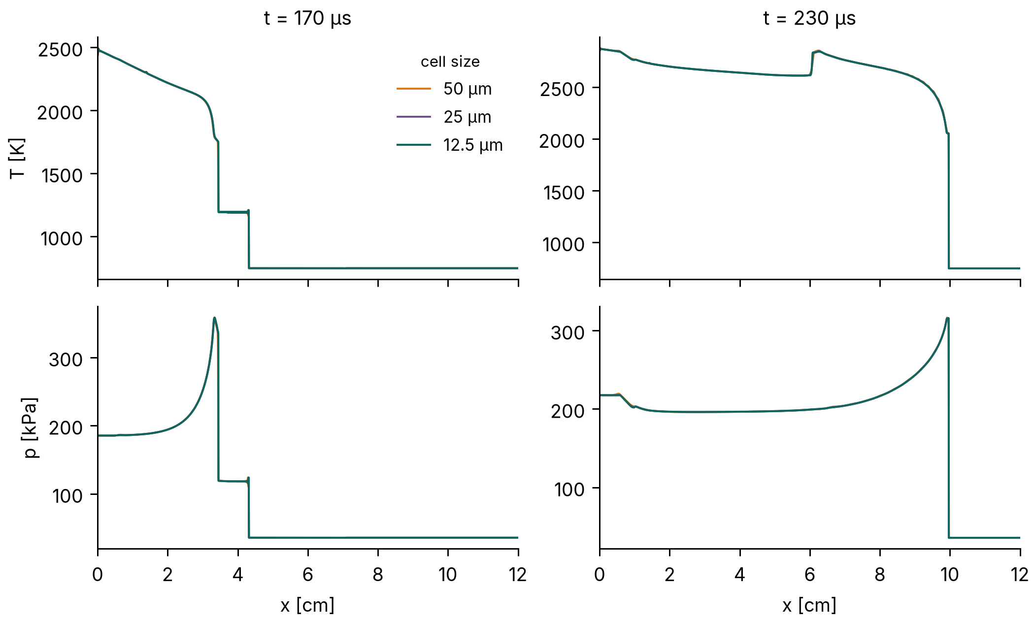
Reactive shock tube in 2H2-O2-7Ar (Fedkiw et al. 1997; Martinez Ferrer et al. 2014): the gas behind the reflected shock ignites and a detonation overtakes the reflected shock; the front at 230 us converges to 99.6 mm under refinement
Size, time on 12 CPU threads: 2,400 cells (50 um); 4,800 and 9,600 for the convergence check. Input file · results
detonation_1d
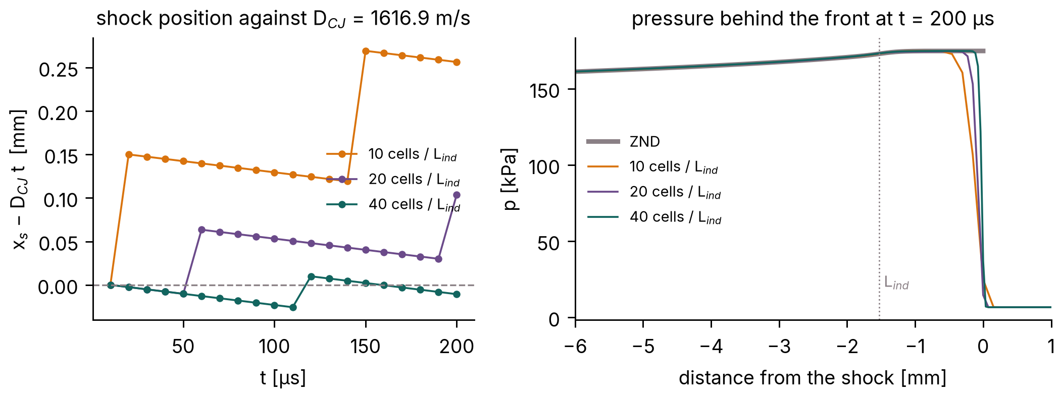
Planar CJ detonation in 2H2-O2-7Ar at 6.67 kPa, started from its ZND structure (generate it with tools/detonation_reference.py and tools/znd_restart.py, see the input's header): the front keeps D_CJ = 1617 m/s within 0.01% at 20 cells per induction length, and the von Neumann pressure
Size, time on 12 CPU threads: 3,934 cells (10 per induction length); 7,868 and 15,736 for 20 and 40. Input file · results
detonation_2d

Cellular detonation in 2H2-O2-7Ar at 6.67 kPa (V9): the ZND detonation of detonation_1d in a 6 cm channel, perturbed by six pockets of fresh gas, with the numerical soot foil (P_MAX); generate the initial state first (see the input's header). Front speed 1617.0 m/s (D_CJ to 0.01%); eight triple points (15 mm cells) thin out to 3 cm cells and fainter tracks over 33 cm of travel; the track pattern is the same at 10 and 20 cells per induction length. tools/soot_foil.py and tools/animate_detonation_2d.py analyze and animate it
Size, time on 12 CPU threads: 1.2M cells, 18,900 steps: 39 minutes on two A100s. Input file · results
detonation_3d
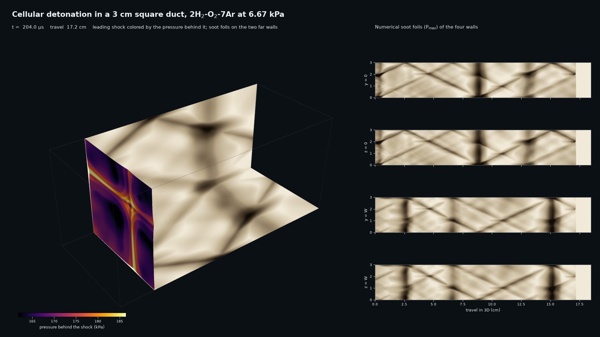
Cellular detonation in a 3 cm square duct (3D build), 2H2-O2-7Ar at 6.67 kPa at 10 cells per induction length, in a window that follows the front (tools/detonation_window.py), started from a 2D cellular detonation (input_2d.toml) turned into in-phase transverse waves in y and z: the rectangular mode with numerical soot foils on all four walls, triple-point tracks and slapping-wave bands; front speed D_CJ to 0.2% over 17 cm. tools/soot_foil_3d.py and tools/animate_detonation_3d.py analyze and animate it
Size, time on 12 CPU threads: 19.2M hexahedra, 12,180 steps: 4.6 hours on four A100s. Input file · results
premixed_flame
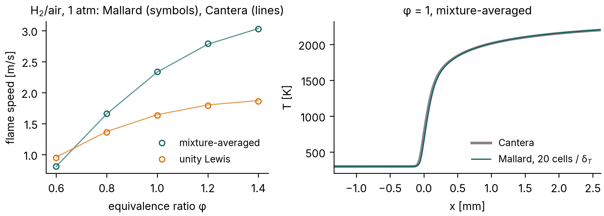
Freely propagating stoichiometric H2/air flame at 1 atm with mixture-averaged transport (V8), started from Cantera's flame in its frame (generate the restart file first, see the input's header); the consumption speed settles within 0.1% of Cantera's 2.332 m/s
Size, time on 12 CPU threads: 300 cells, 20 per thermal thickness, ~10 min on one thread. Input file · results
premixed_flame/ch4
Freely propagating stoichiometric CH4/air flame (GRI-3.0, 53 species) at 1 atm with mixture-averaged transport (V8), started from Cantera's flame in its frame (generate the restart file first, see the input's header); the consumption speed settles 1.3% below Cantera's 0.3758 m/s. tools/flame_sweep.py runs the sweep over phi = 0.6-1.4, both transport models, resolution and CFL
Size, time on 12 CPU threads: 300 cells, 20 per thermal thickness, 445,000 steps: about 2 hours on one A100. Input file
flame_outflow
A stoichiometric H2/air flame blown out through a characteristic outlet, fed by a characteristic inlet: while the flame leaves, the pressure stays within 0.7% of the target and within 0.3% across the domain
Size, time on 12 CPU threads: 60 cells, ~2 minutes on 3 threads. Input file
flame_2d
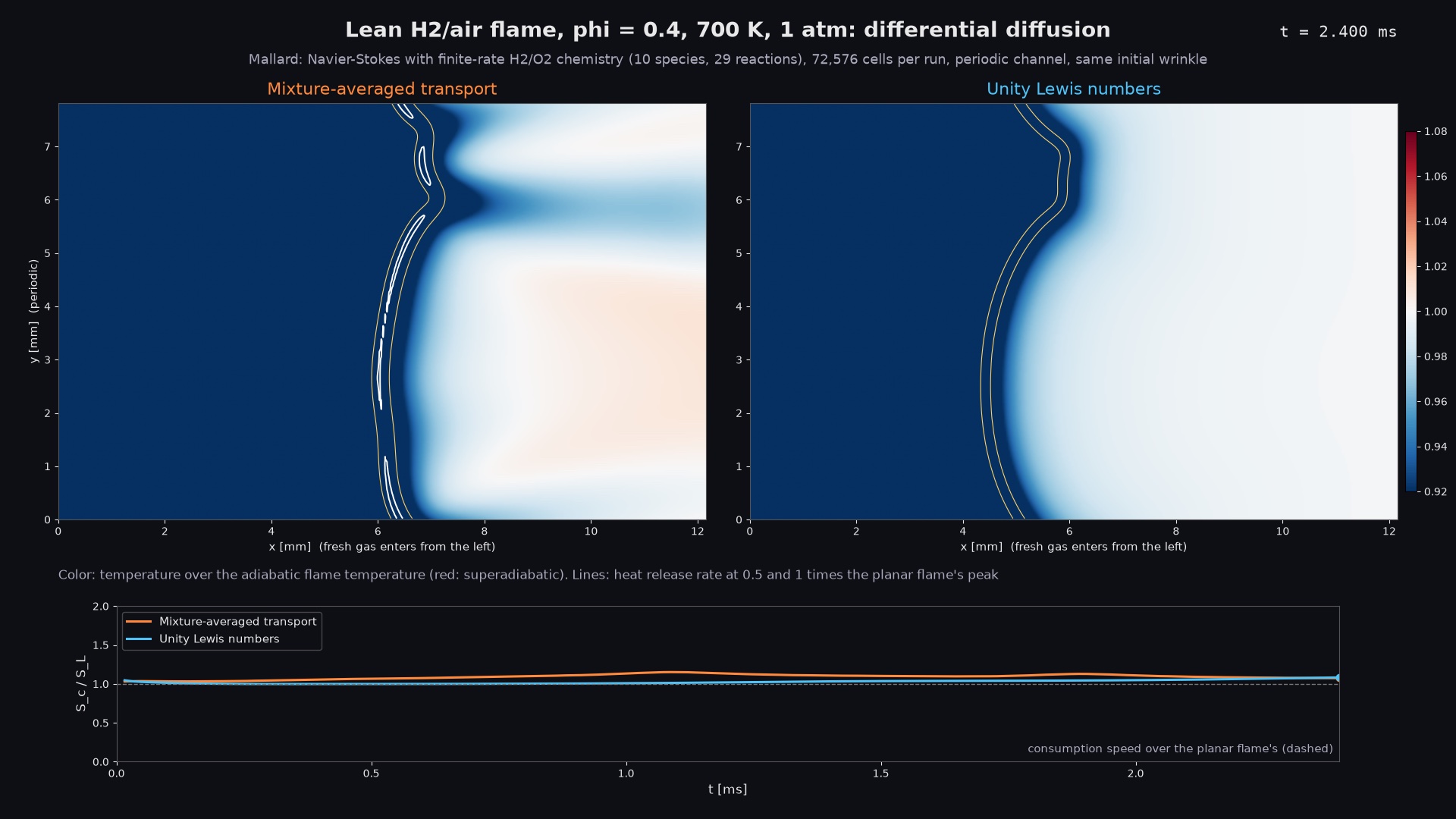
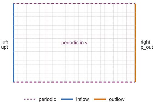
Lean H2/air flame (phi 0.4, 700 K, 1 atm) in a periodic channel with mixture-averaged transport and, in unity/, unity Lewis numbers, from the same wrinkled front: differential diffusion makes the burnt gas 0.96-1.02 times the adiabatic flame temperature (unity Lewis: uniform) and the flame up to 14% faster; planar flames on the same mesh are within 0.6% of Cantera. Generate the initial states first (see the input's header); tools/animate_flame_2d.py animates both side by side
Size, time on 12 CPU threads: 72,576 cells, 300,000-380,000 steps: 70-80 minutes per run on one A100. Input file · results
counterflow_diffusion
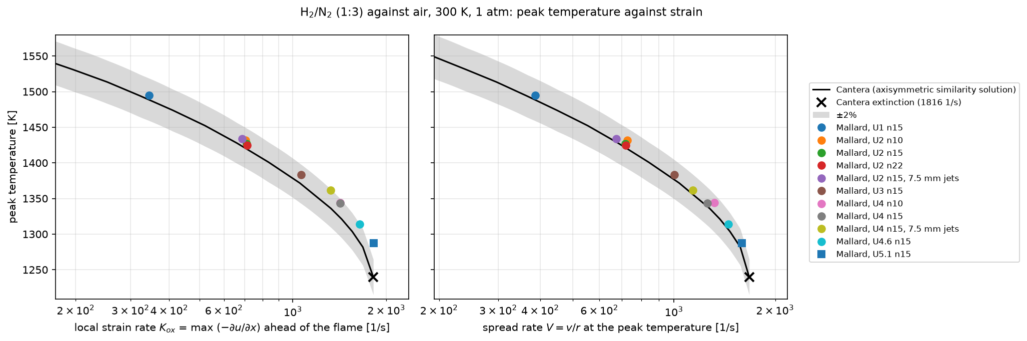
H2/N2 (1:3) against air from opposed round jets, 10 mm apart (V10, 3D build): a quarter domain with N2 coflows, started from Cantera's CounterflowDiffusionFlame (generate the mesh and initial state first, see the input's header and README.md). Peak temperature against local strain rate within 2% of Cantera's from 344 to 1640 1/s (+0.49% at this input's 711 1/s), within 0.6% at matched flame strain; it goes out between 1818 and about 1975 1/s (Cantera: 1816 1/s)
Size, time on 12 CPU threads: 46,464 hexahedra, 15 cells per flame width: 75 minutes on one A100. Input file · results
triple_flame
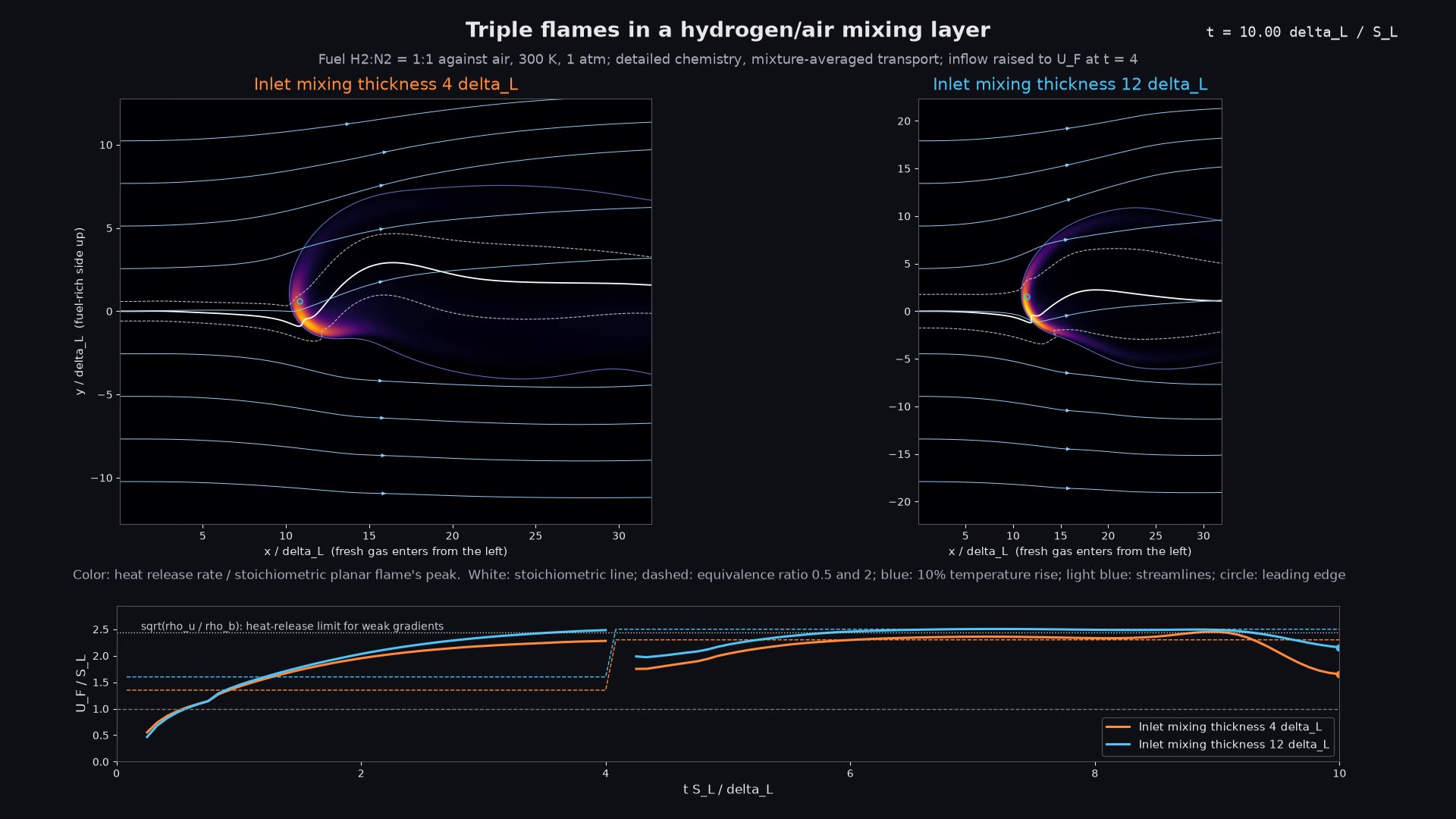
Triple flame of H2:N2 = 1:1 against air at 300 K (mixture-averaged transport) in mixing layers of 4 and, in thick/, 12 thermal thicknesses, against Ruetsch, Vervisch & Liñán (1995): held in place by raising the inflow to its speed, it propagates at UF / SL = 2.31 and 2.46 at local mixing thicknesses DTF = 9 and 28, rising with DTF as theirs (1.23 to 1.51); higher than their one-step, unity-Lewis values because the hydrogen tip burns at 1.24-1.30 SL, while the flow divergence alone gives 1.86-1.90, below √(ρu/ρb) = 2.44. Generate the initial states first (see the input's header); tools/triple_flame_analysis.py and tools/animate_triple_flame.py analyze and animate it
Size, time on 12 CPU threads: 166,000 and 276,000 cells, 12 per thermal thickness, about 330,000 steps: 4 hours per run on two A100s. Input file · results
flame_vortex
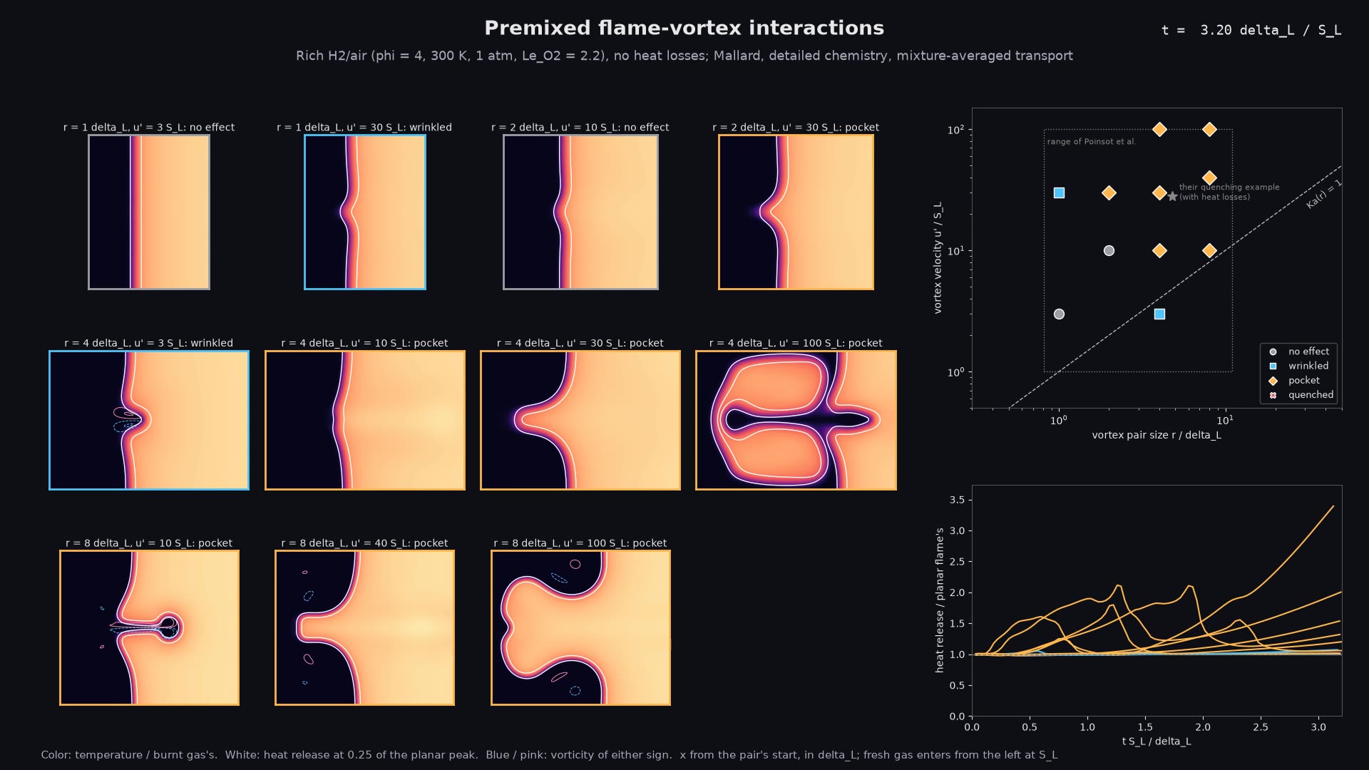
Premixed flame-vortex interactions on the spectral diagram of Poinsot, Veynante & Candel (1991): vortex pairs of 1-8 thermal thicknesses at 3-100 SL against a rich H2/air flame (phi = 4, deficient-reactant Lewis number 2.2, no heat losses). Small pairs fall below the 5% cut-off, larger ones wrinkle the front or cut off pockets of fresh gas, and none quenches, up to Ka(r) = 25 (Poinsot et al.'s quenching needs heat losses: see flame_vortex_quenching). Generate the initial state first (see the input's header); tools/flame_vortex_analysis.py classifies the runs and tools/animate_flame_vortex.py animates them
Size, time on 12 CPU threads: 26,000-85,000 cells, 12 per thermal thickness (24 for the smallest pairs): 12 minutes to 1.5 hours per run on one A100. Input file · results
flame_vortex_quenching
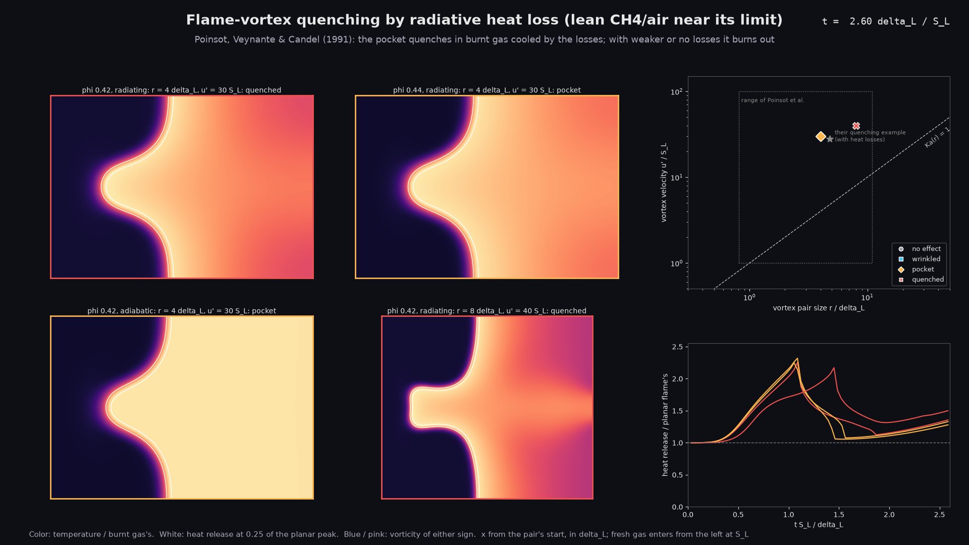
The spectral diagram of Poinsot, Veynante & Candel (1991) with heat losses: vortex pairs of 1-8 thermal thicknesses at 3-100 SL against a lean CH4/air flame near its radiative limit (phi = 0.42, two-step mechanism, optically thin radiation [radiation]). Pairs above a quenching line (Ka(r) between 1.25 and 5 for r = 8 delta_L, rising steeply toward small pairs) cut off a pocket whose downstream side goes out in the radiatively cooled burnt gas, as in their quenching example; the same pair at phi = 0.44 or without radiation leaves a pocket that burns out. Generate the initial state first (see the input's header)
Size, time on 12 CPU threads: 26,000-106,000 cells, 12 per thermal thickness (24 for the smallest pairs): 1-4.5 hours per run on one A100. Input file · results
autoignition_2d
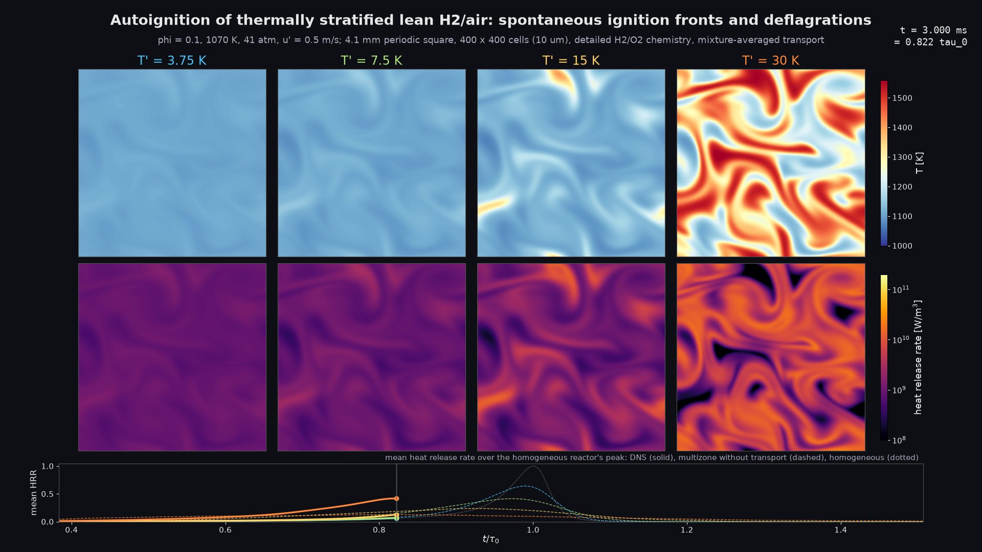
Autoignition of a thermally stratified lean H2/air mixture at constant volume (phi 0.1, 1070 K, 41 atm; Chen et al. and Hawkes et al. 2006, Sankaran et al. 2005): a 4.1 mm periodic square with random temperature fluctuations T' of 3.75-30 K and decaying turbulence, mixture-averaged transport, 11-15 cells per deflagration thickness. Generate the initial state and the 0D references first (see the input's header). Larger T' ignites earlier (mean heat release peak at 0.99 down to 0.82 tau_0) and burns longer (width 0.06 to 0.16 tau_0), and the fronts slow from spontaneous ignition (median 17 S_L) towards deflagration (2.4 S_L, a quarter of the heat release below 1.5 S_L); the multizone model without transport predicts 2-4 times wider bursts, since mixing halves T' before ignition. tools/autoignition_analysis.py and tools/animate_autoignition.py compare and animate the runs
Size, time on 12 CPU threads: 160,000 cells, 1.4-2.0M steps per T': 4.7-5.5 hours on four A100s. Input file · results
shock_bubble_3d
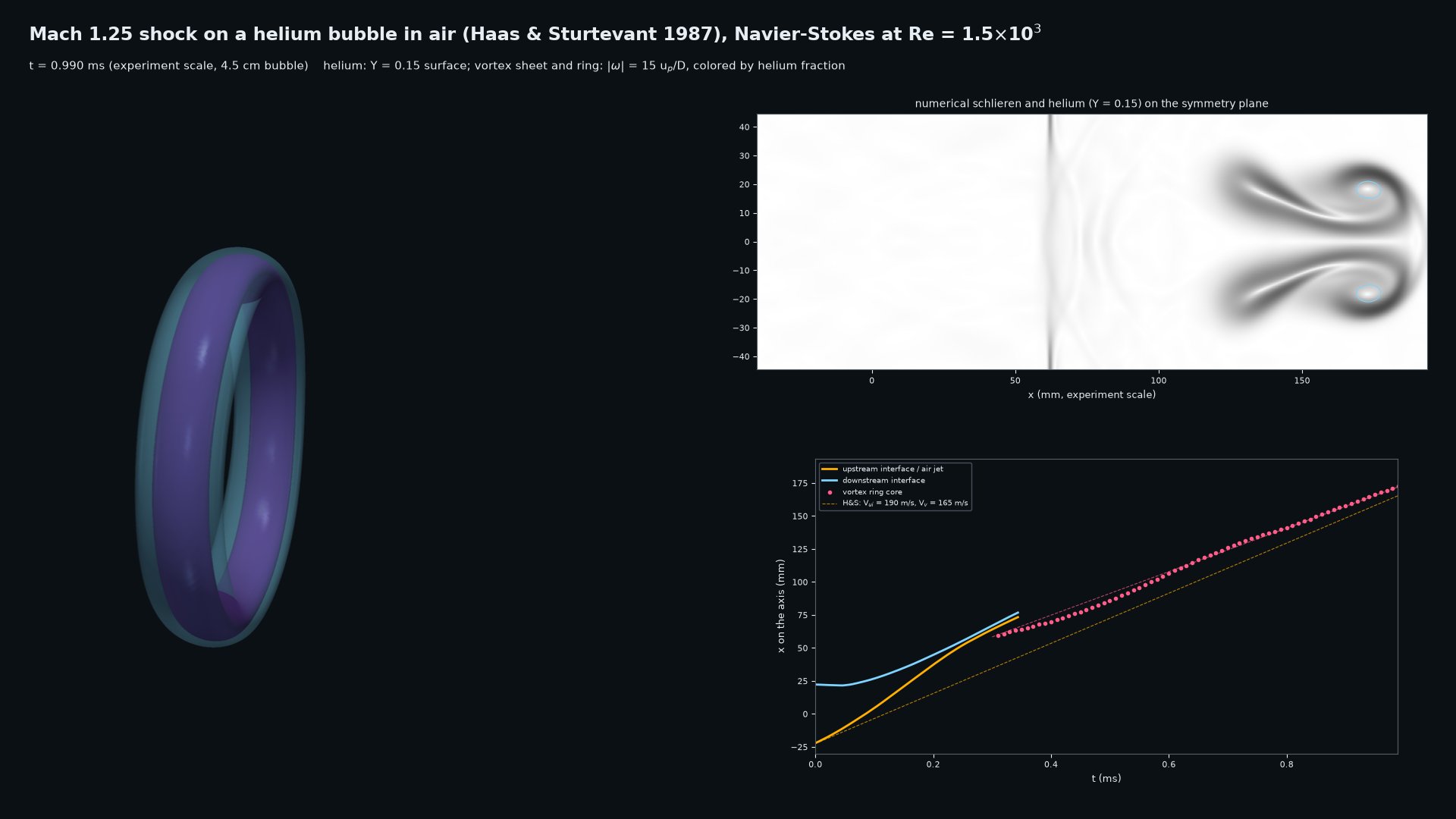
Mach 1.25 shock on a helium bubble in air (3D build; Haas & Sturtevant 1987): Navier-Stokes with mixture-averaged transport at Re = 1.5e3 (the bubble scaled down to 0.18 mm), a quarter of the square shock tube at 128 cells per diameter; the kidney-shaped bubble, the air jet and the vortex ring. Refracted and transmitted shocks, ring and late downstream face within 0-8% of the measured velocities (961, 359, 178, 166 m/s against 960, 365, 165, 165), all within 1.2% at 96 cells per diameter; generate the initial state first (see the input's header); tools/shock_bubble.py compares, tools/animate_shock_bubble.py animates
Size, time on 12 CPU threads: 11.4M hexahedra, 52,091 steps: 3.4 hours on four A100s. Input file · results