Documentation of the main branch
These pages follow Mallard's main branch, which is ahead of release 0.8.0: some features they describe come with the next release.
Design: large-eddy simulation
Status: proposed. Recommendations are marked Decision; the alternatives considered are listed with each. Implementation follows the stages, one pull request each; done: 1, 2, 3, 4, 5 (6 and 7 open:
197, #198).
Mallard resolves every scale it computes today (DNS of flames, detonations, Taylor-Green and isotropic turbulence). This document adds large-eddy simulation (LES) of compressible, possibly reacting, flows with explicit subgrid-scale (SGS) models: an eddy viscosity for the momentum, turbulent Prandtl and Schmidt numbers for heat and species, and a turbulence-chemistry closure for the filtered reaction rates.
Goals
- Explicit models, not implicit LES. Results must be attributable to the models. The scheme's own dissipation is measured at run time and kept below the model's (section 4); validation shows the model-off and model-on runs differ by much more than the model-on runs differ under refinement of the numerical dissipation.
- Unstructured, mixed and high-order meshes: triangles, quadrilaterals, tetrahedra, hexahedra, prisms and pyramids, with any reconstruction (FO, MUSCL, TENO-E of orders 3 to 6).
- Single gases and reacting mixtures: finite-rate chemistry, mixture-averaged / unity-Lewis / constant-Lewis transport, double flux.
- Determinism: results bitwise independent of the MPI rank count and of GPU/CPU team widths, as for the rest of the solver (mpi.md).
- No cost and no change without
[les]: runs without it give byte-identical results and keep their speed. - Validation with literature data and quantitative targets (section 8).
Non-goals
- Implicit LES, or tuning the scheme's dissipation to stand in for a model.
- Wall models (wall-modeled LES). Walls are resolved (y+ of the first cell about 1).
- RANS and hybrid RANS/LES (DES, DDES, WMLES).
- Synthetic inflow turbulence: that is #159. Cases that need it depend on it.
- Flamelet / FPV / FGM tabulated chemistry, transported or presumed PDFs, CMC, linear-eddy models, and other closures built on reduced chemistry manifolds: Mallard's chemistry is finite-rate with mechanisms read at run time, and the closure must keep it.
- SGS models for the isotropic part of the SGS stress, the SGS viscous diffusion, the SGS pressure-dilatation and the triple correlation of the energy equation (section 1).
Summary of decisions
| # | Decision | Main alternatives | Why |
|---|---|---|---|
| 1 | Favre-filtered equations closed by an eddy viscosity mu_t, with lambda_t = cp mu_t / Pr_t and rho D_t = mu_t / Sc_t; mu_t added to the molecular coefficients |
Mixed or scale-similarity models; separate SGS flux kernels | Shares the viscous fluxes, boundary treatment, time step and transport infrastructure; the standard closure of compressible LES (Vreman et al. 1995; Garnier et al. 2009) |
| 2 | Sigma model (Nicoud et al. 2011) as the primary eddy viscosity; WALE, Vreman and Smagorinsky also available | WALE, Vreman, dynamic Smagorinsky as primary | Local, no test filter, positive; vanishes in pure shear, solid rotation, two-component and axisymmetric/isotropic expansion; cubic near walls; insensitive to the one-dimensional dilatation of flames |
| 3 | Dynamic Smagorinsky deferred | Germano-Lilly with local averaging | Needs a test filter and averaging on unstructured mixed meshes (section 2.5); Sigma gets near-wall and laminar behavior without it |
| 4 | Filter width Delta = V^(1/d) (d = 2 or 3) of each cell, independent of the reconstruction order; in 3D times Scotti's anisotropy factor since stage 7 (section 3) |
Largest cell extent; Scotti's anisotropy correction; h / (p + 1) |
A finite volume has one degree of freedom per cell at any order; Sigma and WALE vanish where the cells are most anisotropic (walls) |
| 5 | Eddy viscosity per cell from the viscous cell gradients, averaged to faces; zero on wall faces | Per face from face gradients | One evaluation per cell; enters the time step and output; consistent across ranks |
| 6 | A kinetic-energy budget diagnostic that measures the numerical dissipation of resolved kinetic energy against the SGS and molecular dissipation at run time | Inferring numerical dissipation from -dK/dt after the fact | Proves at every output which term dissipates the energy; needs no reference |
| 7 | A low-dissipation convective flux: a kinetic-energy-preserving (KEEP) central flux blended with the Riemann solver by a compression-only Ducros sensor | Lower TENO cutoff; Riemann solvers with scaled dissipation only; artificial viscosity | Upwind Riemann fluxes dissipate resolved energy at the grid scale at a rate comparable to the SGS model; the KEEP flux adds none, and shocks keep the Riemann solver |
| 8 | Thickened flame (TFLES) with dynamic thickening as the primary combustion closure; since #294 the dynamic efficiency E = F^beta (Charlette et al. 2002; Wang et al. 2011) by default, the Charlette efficiency (beta = 0.5) with Colin's u'_Delta as an option |
PaSR; quasi-laminar | Works with finite-rate mechanisms and molecular transport unchanged; keeps the laminar flame speed exactly; explicit and well validated for premixed LES. Colin's u' doubles S_T at Delta = 1.6 delta_L; the dynamic exponent needs no u' and no constant (section 8.3) |
| 9 | PaSR as an optional second closure, later | None; quasi-laminar | Covers non-premixed and MILD regimes; shares TFLES's per-cell rate scaling |
| 10 | Chemistry rates scaled per cell by advancing each Strang reactor over s dt |
Scaling the rates inside the kinetics | The constant-volume reactor is autonomous, so this is exact; no change to the kinetics or Jacobian |
1. Filtered equations
With the spatial filter \bar{.} (implicit in the grid, width Delta) and the
Favre filter \tilde{f} = \bar{rho f} / \bar{rho}:
d rho/dt      + div(rho u)                                     = 0
d(rho u)/dt   + div(rho u u + p I - tau - tau_sgs)             = 0
d(rho E)/dt   + div((rho E + p) u - (tau + tau_sgs) . u + q + q_sgs) = 0
d(rho Y_k)/dt + div(rho Y_k u + j_k + j_k^sgs)                 = omega_k
(all variables filtered; bars and tildes dropped). The resolved stress
tau, heat flux q and diffusion fluxes j_k are the molecular ones
evaluated with the filtered state; p = rho R T with the filtered mixture
gas constant.
Closures:
- SGS stress,
tau_sgs = -rho (u u~ - u~ u~) = 2 mu_t (S - 1/3 tr(S) I). The isotropic part-2/3 rho k_sgs Iis not modeled: it is absorbed into the pressure. At the turbulent Mach numbers of the validation cases (M_t < 0.3) it is below 1% ofp(Erlebacher et al. 1992; Garnier et al. 2009, chapter 4), and modeling it (Yoshizawa) brings a constant whose value is uncertain. - SGS heat flux,
q_sgs = -lambda_t grad Twithlambda_t = cp mu_t / Pr_t(and, for mixtures, the enthalpy carried by the SGS species fluxes,sum_k h_k j_k^sgs, which is what the molecular energy flux already does withj_k). - SGS species fluxes,
j_k^sgs = -rho D_t (W_k / W) grad X_k + Y_k V_cwithrho D_t = mu_t / Sc_t, added to the molecular mixture-averaged flux in its Hirschfelder-Curtiss form, so the correction velocityV_cmakes the total diffusive fluxes sum to zero to round-off (Poinsot & Veynante 2012, chapter 4). With unity turbulent Lewis number (Pr_t = Sc_t, the default) the SGS enthalpy and species fluxes do not separate enthalpy from composition at subgrid scales. - Neglected: SGS viscous diffusion, SGS pressure-dilatation, SGS
turbulent diffusion of kinetic energy (triple correlation) and the
nonlinearity of
tau(u)andq(T). Vreman, Geurts & Kuerten (1995) showed these are an order of magnitude below the retained terms in mixing layers; the same simplification is used by nearly all compressible LES codes. - Filtered reaction rates
omega_k: section 6.
Decision 1. One eddy viscosity mu_t = rho nu_t per cell; the
molecular viscous kernels use mu + mu_t, lambda + cp mu_t / Pr_t and the
species diffusivities plus mu_t / Sc_t (as rho D_k W_k / W in Mallard's
mole-fraction form). Defaults Pr_t = Sc_t = 0.9; both are inputs.
Alternatives: scale-similarity and mixed models (Bardina; Zang, Street & Koseff) need explicit filtering of the resolved field on the unstructured mesh, with the same test-filter difficulty as dynamic models (section 2.5); gradient (Clark) models are not dissipative enough on their own and need an eddy viscosity anyway. Neither is proposed.
2. SGS eddy viscosity
All models below give nu_t = (C Delta)^2 D(g) from the resolved velocity
gradient g_ij = du_i/dx_j (Vreman's in the form c Delta^2 D(g)), with
S = (g + g^T)/2. In 2D builds g is the 3x3 gradient of a flow with
u_z = d/dz = 0.
2.1 Requirements
An eddy viscosity should vanish where there is no subgrid turbulence and
scale correctly near walls. Properties of a model's D(g) (Nicoud et al.
2011, table I; the entries below are checked in the unit tests, section 7):
| Property | Smagorinsky | WALE | Vreman | Sigma |
|---|---|---|---|---|
| Positive, local, cheap | yes | yes | yes | yes |
| Zero in solid rotation | yes | no | no | yes |
| Zero in pure shear | no | yes | yes | yes |
| Zero for two-component / 2D flows | no | no | no | yes |
| Zero for isotropic expansion | no | yes | no | yes |
| Zero for axisymmetric expansion | no | no | no | yes |
Near-wall nu_t ~ y^3 |
no (y^0) |
yes | no (y^1) |
yes |
| Galilean and rotation invariant | yes | yes | yes | yes |
2.2 Models
- Smagorinsky (1963):
nu_t = (C_s Delta)^2 sqrt(2 S:S),C_s = 0.17(Lilly's value for isotropic turbulence). Kept as the classical reference and for ablations; it needs wall damping, which is not provided. - WALE (Nicoud & Ducros 1999):
nu_t = (C_w Delta)^2 (S^d:S^d)^(3/2) / ((S:S)^(5/2) + (S^d:S^d)^(5/4)),S^d = (g^2 + (g^2)^T)/2 - tr(g^2)/3 I,C_w = 0.5(Nicoud & Ducros recommend 0.5 to 0.6 for isotropic turbulence). - Vreman (2004):
nu_t = c sqrt(B / (a:a))witha_ij = du_j/dx_i,b = Delta^2 a^T a,B = b11 b22 - b12^2 + b11 b33 - b13^2 + b22 b33 - b23^2,c = 2.5 C_s^2 = 0.07. - Sigma (Nicoud, Baya Toda, Cabrit, Bose & Lee 2011):
nu_t = (C_sigma Delta)^2 sigma_3 (sigma_1 - sigma_2)(sigma_2 - sigma_3) / sigma_1^2withsigma_1 >= sigma_2 >= sigma_3 >= 0the singular values ofg,C_sigma = 1.35(calibrated on isotropic turbulence in that paper). The singular values are the square roots of the eigenvalues ofG = g^T g, found in closed form from its invariants (the trigonometric solution of the characteristic cubic, as in the paper's appendix), in double precision.
2.3 Recommendation
Decision 2: Sigma is the primary model (model = "sigma", the default
when [les] is given in 3D).
- It has every property of the table. WALE fails in solid rotation (vortex cores, swirling flows) and Vreman near walls and in rotation; both give an eddy viscosity in laminar two-dimensional regions (e.g. laminar shear layers and flame fronts before transition).
- For reacting flows it is the only one of the four that is zero for the
one-dimensional dilatation across a planar flame (
gof rank one:sigma_2 = sigma_3 = 0). The others turn the thermal expansion of every flame into an eddy viscosity and an SGS diffusivity, which then thickens laminar flames. This also makes the SGS velocity of the combustion closure (section 6.3) free of dilatation. - It costs one 3x3 symmetric eigenvalue problem in closed form per cell, negligible next to the reconstruction.
- It needs no test filter, no averaging and no extra transported field, so it is local, deterministic across ranks and restartable from the state.
Known limitations: Sigma vanishes for all two-dimensional flows, so 2D builds (which cannot hold 3D turbulence anyway; they are for tests and laminar cases) should use WALE or Vreman, and the 2D default is WALE. Its constant is calibrated on isotropic turbulence; Nicoud et al. found the same constant adequate for channel flow, and section 8 checks it.
WALE is the fallback in 2D and the comparison model in validation. Vreman is the cheapest and is kept for comparison with the literature, where it is common. Smagorinsky is for ablation studies: it shows what the near-wall and laminar properties buy.
2.4 Rejected or deferred alternatives
- Anisotropic minimum-dissipation (AMD) (Rozema et al. 2015): attractive
for anisotropic grids (it uses directional filter widths), but its
nu_t = max(0, ...)clips half of the configurations and its constant depends on the discretization order. Possible later addition; not needed for the recommended validation. - Dynamic Smagorinsky (Germano et al. 1991; Lilly 1992; for compressible flow Moin et al. 1991): Decision 3, deferred. See below.
2.5 Why not the dynamic Smagorinsky model (yet)
The Germano identity L_ij = T_ij - \hat{tau}_ij determines C_s^2(x, t) from
the resolved field filtered at a test scale \hat{Delta} > Delta. On
Mallard's meshes:
- The test filter. A discrete filter on an unstructured mixed mesh (e.g.
a volume-weighted average over vertex neighbors) has a transfer function
that depends on the local cell type and arrangement, so its width
\hat{Delta}/Delta, which entersM_ijdirectly, is not uniform: it differs between hexahedra (27-cell stencil), tetrahedra (up to about 100 vertex neighbors) and prisms. Commutative and well-defined unstructured filters exist (Haselbacher & Vasilyev 2003; Najafi-Yazdi, Najafi-Yazdi & Mongeau 2015), but they are wide, need per-cell weights computed at setup, and still give a mesh-dependent effective ratio at mesh transitions. - Averaging. The raw coefficient
C = <L:M> / <M:M>is negative over large regions and must be averaged. Plane or line averages need homogeneous directions, which general meshes lack. The alternatives are local volume averaging (another filter, with the same issues) or Lagrangian averaging (Meneveau, Lund & Cabot 1996), which adds two transported fields with their own advection scheme, restart variables and relaxation time. - Clipping (
nu + nu_t >= 0) is still required, and makes the model partly ad hoc. - Cost and halo depth: two extra filter passes per stage over 10 to 20 quantities, each widening the halo the eddy viscosity needs by one layer.
Sigma achieves the main benefits of the dynamic procedure (zero
nu_t in laminar and near-wall regions, correct y^3) locally. A dynamic
Sigma or dynamic Smagorinsky with Lagrangian averaging can follow if
validation shows the static constant is inadequate (stage 7).
As implemented (stage 7, opt-in dynamic = true): a global dynamic
procedure. Section 8.1 showed the best static constant depends on the
resolution (1.8 at 64^3, 1.35 at 128^3), which is what a dynamic constant
should capture. The global form (one constant per step, C^2 = <L^d:M> /
<M:M> summed over the domain) avoids the averaging and clipping problems
above, and its test filter, the volume-weighted average over a cell and its
vertex neighbors, enters only through Delta_hat^2 = Delta^2 + 12 / d
tr(cov) of each cell's own stencil (3 Delta on uniform hexahedra), so
mesh transitions are handled cell by cell. Favre-weighted L and M (Moin
et al. 1991), filtered gradients for the gradients of the filtered field.
The sums are exact (fixed point, scaled to the largest term), so the constant
does not depend on the rank count. Cost: one extra pass over the vertex
neighbors per step (about 30% of a CPU step on the CBC case, once per step).
| Case | static C |
dynamic C (time mean) |
result, dynamic vs static 1.35 |
|---|---|---|---|
| CBC 32^3 | 1.35 / 1.8 | 1.6 (rising from 1.1) | spectral error 0.165 / 0.142 vs 0.153 / 0.151 (1.8: 0.103 / 0.082) |
| CBC 64^3 | 1.35 / 1.8 | 1.4 | 0.116 / 0.077 vs 0.107 / 0.104 (1.8: 0.058 / 0.063) |
| CBC 128^3 | 1.35 / 1.8 | 1.15 | 0.060 / 0.054 vs 0.063 / 0.085 (1.8: 0.124 / 0.141) |
| channel 395, 64^3 | 1.35 | 1.09 | Re_tau 408.0 (+4.0%) vs 402.3 (+2.6%); peak v_rms+ 0.912 vs 0.889 |
The procedure finds the right trend with resolution (1.6, 1.4, 1.15) and the
best spectra of any run at 128^3, but not the 1.8 that fits 64^3: that
optimum compensates the second-order scheme's damping near the cutoff,
which the Germano identity, written for the filter alone, cannot see. In the
channel the domain-wide constant is pulled down by the regions of weak SGS
activity and the mean flow is worse than with the static constant. Hence
opt-in, not the default. eps_num / eps_sgs stays below the criterion
(CBC 0.006-0.04, channel 0.40).
3. Filter width
Decision 4. Delta = V^(1/d): the cube root of the cell volume in 3D
(Deardorff 1970), the square root of the cell area in 2D (the planar area in
axisymmetric runs), for every cell type and reconstruction order.
- High order. In a finite volume method each cell carries one average
whatever the reconstruction order, so the shortest resolved wavelength is
about
2 hat every order; a higher-order reconstruction resolves more accurately the scales near that cutoff rather than smaller ones.h / (p + 1), the width used for discontinuous Galerkin and spectral-element LES where a cell carries(p + 1)^ddegrees of freedom, does not apply. Low-order schemes damp a band below the cutoff, i.e. act as an additional implicit filter; this is what the dissipation budget (section 4) measures, rather than a factor folded into Delta. - Anisotropy. Deardorff's width underestimates the largest extent of
stretched cells. Scotti, Meneveau & Lilly (1993) give a correction
f(a_1, a_2) = cosh(sqrt(4/27 ((ln a_1)^2 - ln a_1 ln a_2 + (ln a_2)^2)))of the aspect ratios; the largest extent (Delta_max) is used in DES. Both matter most in wall cells, where Sigma and WALE are already small (y^3); the Scotti factor is 1.2 for an aspect ratio of 5 and 1.4 for 10. Implemented (stage 7) asfilter_width = "scotti", the default in 3D, with each cell's extentsh_i = V / lambda_ifrom the eigenvalues of its projected-area tensor1/2 sum_f A_f A_f^T / |A_f|(exact for boxes, face data only, so periodic cells need no unwrapping), for the eddy viscosity only (TFLES keepsV^(1/3)). Channel atRe_tau = 395, 64^3, Sigma 1.35:Re_tau394.8 (+0.7%, against +2.6% withV^(1/3)),Cf+0.9%,U+at y+ = 30 / 100 13.40 / 16.61 (MKM 13.49 / 16.53),eps_num / eps_sgs0.21; peakv_rms+0.882, unchanged. AtRe_tau = 590(96^3, section 8.2):Re_tau596.6 (+1.6%) against 611.0 (+4.1%) withV^(1/3),Cf+2.9% against +7.9%,U+at y+ = 30 / 100 13.33 / 16.43 (MKM 13.53 / 16.54). On cubic cells it isV^(1/3), so the isotropic turbulence and flame cases are unchanged. Hence the default in 3D (2D keepsV^(1/2)). - Mixed meshes.
V^(1/d)is continuous across hexahedron-prism- tetrahedron transitions of equal edge length up to the volume ratio's cube root (a regular tetrahedron of edge h hasV^(1/3) = 0.49 h, a cubeh): tetrahedral regions get a smaller Delta at the same edge length, which is consistent with their higher number of cells per volume.
4. Keeping the model's dissipation dominant
4.1 The problem
Mallard's convective flux is an approximate Riemann solver applied to
high-order reconstructed states (TENO-E, MUSCL). Its upwind part dissipates
kinetic energy at a rate proportional to |lambda| (u_R - u_L)^2, where the
jump u_R - u_L of the reconstructions is O(h^p) for smooth fields but
O(1) relative at the grid cutoff, precisely where the SGS model acts
(Ghosal 1996; Mittal & Moin 1997; Garnier et al. 1999). Two further sources:
- TENO-E's nonlinear stencil selection discards the central stencil in
troubled cells, and on LES meshes most cells near the cutoff are flagged
(76% of cells at 64^3 in
examples/isotropic_turbulence), so the reconstruction falls back to more dissipative sector stencils. - The low-Mach correction (Thornber et al. 2008) already scales the velocity
jump by
min(1, max(M, M_cut)), so atM ~ 0.1the upwind dissipation of the velocity field is reduced roughly tenfold; it does not remove it.
In under-resolved turbulence these terms can match or exceed the SGS dissipation. Then the results are implicit LES, whatever model is switched on. The design therefore (a) measures the numerical dissipation at run time, and (b) provides a convective flux that adds none in smooth regions.
4.2 Dissipation budget (decision 6)
The semi-discrete rate of change of the resolved kinetic energy
K = sum_c V_c rho_c |u_c|^2 / 2 caused by any part R of the right-hand
side (R_rho, R_m per cell, conservative form) is exactly
Mallard evaluates it separately for the convective, molecular viscous and SGS fluxes (one extra RHS evaluation, at the output interval only). For a periodic or walled domain the exact (continuous) contributions are
- convection:
Pi = int p div u dV(pressure-dilatation work; transport terms integrate to zero), - molecular viscosity:
-eps_mol = -int tau : grad u dV, - SGS:
-eps_sgs = -int tau_sgs : grad u dV.
The numerical dissipation is then eps_num = Pi_h - dK/dt|_conv, with
Pi_h the scheme's own pressure work: on interior faces, the work of the
two-point pressure flux mean(p) n of the cell values, sum_f mean(p) (u_1 -
u_0) . n A_f (a central flux with first-order states changes K by exactly
this, section 4.3), plus the whole kinetic-energy rate of the boundary faces'
fluxes, so that eps_num is the dissipation of the interior faces. The run
reports eps_mol, eps_sgs, eps_num, Pi_h (pressure_work) and Pi
from the cell gradients (pressure_dilatation) in [integrals] (with
budget = true). The criterion
for an LES result to count as explicit-model LES is eps_num <= 0.5 eps_sgs
averaged over the analysis window, i.e. the model removes at least two
thirds of the energy that leaves the resolved scales through the cutoff.
eps_num includes the reconstruction's and the Riemann solver's dissipation
together (dK/dt of the convective operator, whatever causes it); the time
integrator's dissipation (SSPRK3's, of order (lambda dt)^4) is not
included and is negligible at the CFL numbers used.
Why the discrete pressure work: until #197 eps_num was Pi - dK/dt|_conv
with Pi from the cell gradients, exact only up to their discretization
error. That is harmless where |Pi| is a few percent of the dissipation
(isotropic turbulence and the channel at M_t <= 0.2: on the 64^3 CBC case
with Sigma C = 1.8 the numerical share is -0.9% with Pi_h against +0.7%
with Pi), but not in a flame at 1 atm, where thermal expansion makes p
div u 1e3 to 1e4 times the dissipation and the gradient estimate of Pi
then measures its own error (initial state of a coarse run of section 8.3's
flame: Pi = 18.6 W from the gradients, dominated by the gas leaving
through the outlet at 1 atm, against Pi_h = 0.022 W, dK/dt|_conv =
0.024 W and an SGS dissipation of 0.0014 W). Pi_h uses the same face pressures and cell velocities as the
convective operator, so constant pressure cancels exactly and the open
boundaries' fluxes (an outlet's p u . n) drop out.
4.3 Low-dissipation convective flux (decision 7)
[numerics] convective_flux = "hybrid" replaces the Riemann flux by
at every face quadrature point, with the same reconstructed states.
F_KEEPis the kinetic-energy- and entropy-preserving two-point flux of Kuya, Totani & Kawai (2018): with arithmetic means\bar{.},C = \bar{rho} \bar{u}.n, massC, momentumC \bar{u} + \bar{p} n, energyC (\bar{e} + u_L . u_R / 2) + (p_L u_R.n + p_R u_L.n) / 2. For a mixture,e = p / ((gamma - 1) rho) + e0per side with the face's surrogates. Its momentum flux has Jameson's (2008) formC \bar{u} + \bar{p} nwith the mass fluxC, so for cell values (W_L, W_Rthe two cells' averages) the semi-discrete kinetic energy changes only by the pressure work, on any mesh: per face,(u_R - u_L) . (C \bar{u} + \bar{p} n) - C (|u_R|^2 - |u_L|^2) / 2 = \bar{p} (u_R - u_L) . n. With high-order reconstructed states this holds to the reconstruction's accuracy.phi_f = max(phi_c0, phi_c1)from a cell sensor: the Ducros et al. (1999) sensor restricted to compressions (Bhagatwala & Lele 2009),theta = H(-div u) (div u)^2 / ((div u)^2 + |omega|^2 + eps), andphi_c = 1wheretheta > theta_*(default 0.65), elsephi_min(default 0). Shocks therefore keep the full Riemann solver and TENO's shock-capturing; vortical and expansion regions, and flames (expansions), get the central flux.- Species stay upwinded by the mass flux (Larrouturou) with the blended mass flux, so mass fractions stay in [0, 1] and sum to one; their numerical diffusion is not part of the kinetic-energy budget and is reported separately in validation via scalar variance decay where relevant.
- The low-Mach correction acts on the Riemann part only.
- Double flux: the blend applies to both of a face's fluxes, each central flux with its own side's frozen thermodynamics on both sides.
- Boundary faces other than walls and symmetry planes (whose mirror ghost states make the central flux exact: no mass flux, the pressure force) keep the Riemann solver.
- As implemented (stage 2): contacts and expansions are central, so on Sod's problem (MUSCL, 200 cells) the L1 density error is 1.8 times the Riemann solver's, with a 0.1% overshoot at the contact; without the sensor (central everywhere) the shock oscillates and the error is more than twice the hybrid's. With first-order reconstruction the convective kinetic-energy rate equals the pressure work to round-off on triangles and tetrahedra (tested).
Stability. The central flux has no dissipation, so the SGS model and the molecular viscosity are the only sinks at the cutoff, which is the intended LES. KEEP-type fluxes are stable for turbulence on smooth meshes (Kuya et al. 2018; the same form underlies the second-order central schemes of production LES codes on unstructured meshes). The residual risk is aliasing on very irregular meshes or with nonlinear TENO stencils; `phi_min
0` (e.g. 0.05) is the documented remedy, and the budget reports the dissipation it adds.
Alternatives considered:
- Lowering TENO's dissipation (fixed small
C_T, smallerstencil_factor,troubled_thresholdup): reduces but never removes the upwind dissipation of the Riemann solver, and makes shock capturing less robust everywhere. Useful in combination; the budget quantifies it. - Scaling only the Riemann solver's dissipation (e.g. Roe with its
dissipation matrix multiplied by
phi): equivalent to the blend above for Rusanov and close to it for Roe, but tied to one solver; the blend works with all five. - Artificial bulk viscosity (localized artificial diffusivity, Cook & Cabot) for shocks with a central flux everywhere: needs second derivatives and tuned constants, and is itself numerical dissipation that the budget would have to separate.
- Implicit LES (no model, rely on TENO/Riemann dissipation): a non-goal.
5. Implementation: SGS fluxes in the solver
- Input
[les]:model(sigma,wale,vreman,smagorinsky), optionalC,Pr_t,Sc_t.[les]needstype = "navier_stokes". les.h: the models as one POD withKOKKOS_INLINE_FUNCTION nu_t(g, Delta), captured by value likeEuler.Deltaper cell, computed once at setup (V^(1/d)).- SGS coefficients per cell,
[mu_t, lambda_t, mu_t / (Sc_t W)](les_coefficients), computed after the viscous gradients of each RHS on all local cells, so halo cells next to owned faces have them from the same gradients as their owners. Single gases takelambda_t = cp mu_t / Pr_twith the constantcp; mixtures each cell'scp(T, Y)and mean molar massW. - Viscous fluxes:
ViscousFluxFunctorandMixtureViscousFluxFunctoradd the face means of the SGS coefficients tomu, the conductivity and (mixtures) every species'rho D_k W_k / W(asW_k mu_t / (Sc_t W)). The molecular coefficients and their output (MU,LAMBDA,D_k) are untouched. Wall faces get no SGS flux (the wall shear stress and heat flux are molecular; Sigma and WALE areO(y^3)there anyway); other boundary faces take the cell's value. - Time step: single gases use
max(4/3 (mu + mu_t), gamma (mu / Pr +
  mu_t / Pr_t)) / rho
; mixtures grownu_effbymax(4/3 nu_t, lambda_t / (rho cv), nu_t / Sc_t). The eddy viscosity is recomputed from the state incalc_dt(one gradient evaluation per step), so a restarted run takes exactly the time steps of the uninterrupted one. - Axisymmetric runs are not supported (LES of turbulence is
three-dimensional; the hoop terms would need
mu_tin the reconstruction's geometric source). - Output:
MU_T(cell eddy viscosity). - Budget:
[integrals] budget = trueadds the columnske_rate_convective, ke_rate_viscous, ke_rate_sgs(thedK/dt|_Rof section 4.2) andeps_numerical = pressure_dilatation - ke_rate_convective, from one extra RHS evaluation that neither updates the mixture temperature seeds nor advances the characteristic boundaries, so output does not change the solution. - Without
[les]no new kernel runs and no view is allocated; the existing kernels take the empty-view branch, so results are byte-identical.
6. Turbulence-chemistry interaction
6.1 The candidates
The filtered rates \bar{omega}_k must be modeled because on an LES mesh the
flame (thermal thickness delta_L ~ 0.1-0.5 mm for hydrocarbon and hydrogen
flames at 1 atm) is thinner than Delta (1-5 mm in a laboratory burner LES).
| Closure | Idea | With finite-rate mechanisms | Explicit? | Premixed | Non-premixed |
|---|---|---|---|---|---|
| Quasi-laminar | omega(\tilde{Y}, \tilde{T}) |
yes | no: an under-resolved flame is thickened by the scheme | DNS-like meshes only | if mixing is resolved |
| TFLES (Butler & O'Rourke 1977; Colin et al. 2000) | thicken the flame by F so it is resolved; restore the SGS wrinkling by an efficiency E |
yes, unchanged | yes | yes, the standard premixed LES closure | only with the thickening switched off there (dynamic) |
| PaSR (as in Sabelnikov & Fureby 2013) | omega = kappa omega(\tilde{Y}, \tilde{T}), kappa = tau_c / (tau_c + tau_mix) |
yes | yes, but tau_c is ill-defined for multi-step chemistry |
flame still under-resolved unless the mesh resolves it | yes |
- Quasi-laminar (no model) is the model-off baseline. On an LES mesh it is implicit: the resolved flame thickness is set by the scheme's dissipation and the cell size. Rejected as the closure; kept as the reference that shows what the model changes.
- TFLES: the transformation
D -> F D,omega -> omega / Fkeeps the laminar flame speeds_L ~ sqrt(D omega)and multiplies the thickness byF, for any mechanism and transport model, because it is an exact rescaling of the one-dimensional flame equations. The efficiencyE >= 1(D -> E F D,omega -> E omega / F) multiplies the speed byE, the SGS flame-surface wrinkling. Dynamic thickening (Légier et al. 2002) appliesFonly in the flame through a sensorOmega, so mixing and non-reacting regions keep their molecular and SGS transport. - PaSR: local, cheap, used for non-premixed and MILD combustion; but it
does not resolve the flame structure (the flame is still thinner than the
mesh, so its propagation is again set by numerics in premixed regimes),
and
tau_cfor a multi-step mechanism (from the Jacobian's eigenvalues, from fuel consumption, from a reference flame) changes the results by tens of percent.
6.2 Recommendation
Decision 8: TFLES with dynamic thickening and the Charlette efficiency is the primary closure. It keeps the finite-rate chemistry and the molecular transport models as they are, so the laminar flame speed, thickness ratio and response to strain are those of the mechanism; it is explicit (every effect is a term with a model constant); and its premixed validation is extensive (Colin et al. 2000; Charlette et al. 2002; Wang, Boileau & Veynante 2011; Volvo and swirl burners in AVBP).
Decision 9: PaSR is worth adding as a second closure for non-premixed
and partially premixed cases, but after TFLES is validated. It reuses
TFLES's per-cell rate scaling (section 6.4) and the SGS mixing time
tau_mix = Delta^2 / nu_t from section 2, so it costs about one stage.
6.3 TFLES formulation
Per cell, frozen over a time step (computed at the start of each step from the current state, so restarts reproduce):
- Thickening
F = 1 + (F_max - 1) OmegawithF_max = max(1, n_res Delta / delta_L):n_res(default 5) cells across the thickened flame,delta_Lthe laminar thermal thickness (input; e.g. from Cantera's 1D flame,(T_b - T_u) / max |dT/dx|). - Sensor
Omegain [0, 1]: from the progress variablec = (T - T_u) / (T_b - T_u)clipped to [0, 1],Omega = min(1, c (1 - c) / (c_0 (1 - c_0)))withc_0 = 0.05: one in the whole flame including its preheat zone, zero in fresh and burnt gas.T_uandT_bare inputs. It is local (no filtering pass, so no halo exchange) and smooth. Alternatives: the reaction-rate sensor of Légier et al. (Omega = tanh(beta omega / omega_max), filtered to widen it over the preheat zone, which needs a filtering pass and a halo exchange per step), and Jaravel's multi-step variant; the temperature-based sensor is chosen for its locality and because it cannot fire in non-reacting mixing of cold streams. Its weakness, heat loss loweringcin burnt gas, is not present in the validation cases. - Efficiency (Charlette, Meneveau & Veynante 2002, with
beta = 0.5):E = (1 + min[F - 1, Gamma(F, u'_Delta / s_L, Re_Delta) u'_Delta / s_L])^betawith the filter width of the thickened flameDelta_e = F delta_L, so the ratioDelta_e / delta_L = F;Gammais their fit of the efficiency function, andRe_Delta = u'_Delta Delta_e / nu. In unthickened regions (F = 1)E = 1. - SGS velocity
u'_Delta = c_2 Delta^3 |lap(curl u)|withc_2 = 2(Colin et al. 2000), which removes the dilatational part of the resolved field near the flame. The Laplacian of the vorticity is the divergence of its least-squares gradient: two more gradient passes than the eddy viscosity. It is evaluated on owned cells and its result (F,E,Omegaper cell) is exchanged once per step to the halo. Alternative:u'_Deltafrom the eddy viscosity (nu_t / (C Delta)), which with Sigma is also dilatation-free for planar flames, local and cheaper; kept as an option if the Laplacian proves noisy on tetrahedra. - Dynamic efficiency (
efficiency = "dynamic", the default since #294; Charlette, Meneveau & Veynante 2002, part II; Wang, Boileau & Veynante 2011): Charlette's saturated power law atDelta_e = F delta_L,E = (Delta_e / delta_L)^beta = F^beta, withbetafrom the flame-surface identity between the combustion filter and a test filter of widthgamma Delta_e: the total surface is the same at both widths,<E_Delta |grad c|> = <E_gamma Delta |grad hat(c)|>, so withbetauniformgamma^beta = <hat(|grad c|)> / <|grad hat(c)|>.cis the sensor's progress variable;|grad c|its least-squares gradient on the vertex-neighbor stencil. The test filter isnpasses of the volume average over the cell and its vertex neighbors (the dynamic SGS procedure's filter, section 2.5), each of squared width12 / d tr(cov)(8 h^2on cubes);n(fixed at setup) is the smallest that makesntimes that width reachDelta_e^2on average over the thickened cells (4 on uniform hexahedra atn_res = 5), and each cell'sgamma^2 = 1 + n width^2 / Delta_e^2(Delta_e = F_max delta_L; 1.51 on cubes). The averages<.>are global, over the cells the mesh thickens (F_max > 1), summed exactly in fixed point like the dynamic SGS constant, sobetadoes not depend on the rank count;ln gammaenters|grad hat(c)|-weighted.betais clipped to [0, 1] (fractal dimension 2 to 3), and 0 when no flame is resolved (resolved surface below 1e-6 of the thickened volume overDelta_e: round-off of a uniform field), so it is a function of the state alone and restarts reproduce. No subgrid velocity and no constant: a flat resolved flame givesbeta = 0andE = 1. Cost per step: one gradient ofc,nfilter passes with a halo exchange each, one gradient ofhat(c)and one fixed-point reduction of four sums (the Colin operator's two vorticity passes are skipped). The integrals file gets atf_betacolumn. - Transport: species diffusivities and the conductivity become
E F D_kandE F lambda, and the SGS diffusivities(1 - Omega) D_t(the thickened flame is resolved, so its SGS transport is inE); viscosity is not thickened. - Chemistry: rates
E omega / F, see 6.4. - Inputs (
[les.combustion]):model = "tfles",delta_L,s_L,T_unburnt,T_burnt, optionaln_res(5),efficiency = "dynamic" | "charlette" | "none"; withcharlette,beta(0.5),subgrid_velocityandC_u.
6.4 Chemistry rate scaling (decision 10)
Mallard's chemistry is Strang split: each owned cell is an adiabatic,
constant-volume reactor dY/dt = omega(Y, T)/rho. That system is
autonomous, so multiplying the rates by s is identical to integrating it
over s dt instead of dt. TFLES (s = E / F) and PaSR (s = kappa)
therefore only need a per-cell multiplier of the reactor's integration time.
The kinetics, Jacobian, Rosenbrock integrator, sub-step history (CHEM_H),
skipping of inactive cells and team-parallel lanes are untouched, so the
chemistry stays bitwise independent of rank count and team width.
6.5 Compatibility
- Mixture-averaged, unity- and constant-Lewis transport: thickening
multiplies each
D_kandlambdaby the same factor, so Lewis numbers are unchanged. - Double flux: concerns only the convective energy flux; independent.
- Determinism:
F,E,Omegaare per-cell functions of the state and of its gradients over the local stencil, exchanged to the halo by the same exchange as the state; the result is bitwise independent of the rank count. The only reduction, the dynamic efficiency's four domain sums, is exact in fixed point.
6.6 As implemented (stage 5)
F,E,OmegaandE / Fare computed incalc_dt(once per step, from the state, so restarts reproduce) on owned cells: the vorticity from the transport gradients, exchanged to the halo, its least-squares gradient, and its Laplacian as the divergence of the face gradients (cell means corrected along the line of centroids, no flux through boundary faces); the fields are then exchanged to the halo (two exchanges of three values per cell and step).- The thickening multiplies
LAMBDA, everyrho D_k W_k / Wand the time step'snu_effbyE Fafter the eddy viscosity of each RHS, and the SGS heat and species coefficients by1 - Omega; viscosity is unchanged. HRRandOMEGA_*outputs are the modeled rates (timesE / F).- The SGS model in 2D builds should be Vreman for flames: WALE's eddy viscosity is not zero for the one-dimensional dilatation across a flame.
- Results, one-dimensional stoichiometric H2/air flame (h2o2.yaml,
mixture-averaged,
s_L = 2.3324m/s,delta_L = 0.330mm from Cantera), MUSCL and HLLC, strip cells of aspect ratio 10 (Delta = 3.16 dx),n_res = 5:
| Mesh | Model | F |
Consumption speed | Displacement speed | Thermal thickness |
|---|---|---|---|---|---|
2 cells per delta_L |
TFLES | 7.91 | 2.327 m/s (-0.2%) | 2.291 m/s (-1.8%) | 2.615 mm (F delta_L = 2.610 mm) |
0.5 cells per delta_L |
TFLES | 31.6 | 2.328 m/s (-0.2%) | 2.251 m/s (-3.5%) | |
0.5 cells per delta_L |
none (quasi-laminar) | 1 | 2.273 m/s (-2.5%) | 2.240 m/s (-4.0%) | one cell (numerical) |
The thickened flame keeps the laminar speed and has the thickness F
delta_L it is designed to have; the quasi-laminar flame's speed is also
within 5% in this one-dimensional case, but its structure is one cell
wide, set by the scheme. The displacement speeds include the slow drift
of a long domain's flame position (they are fitted over the last half of
the run). The thickened post-flame recombination zone is F times longer
too (rates times 1 / F while c < 0.95), so the peak temperature in a
domain of a few thickened thicknesses stays below the adiabatic one
(2224 K against 2384 K at F = 7.9).
7. Tests (each must fail under a plausible bug)
- Model kernels (exact values): Sigma, WALE, Vreman, Smagorinsky on
analytic gradients: pure shear (WALE, Vreman, Sigma give 0;
Smagorinsky
(C Delta)^2 |s|), solid rotation (Smagorinsky and Sigma give 0, WALE and Vreman positive), isotropic and axisymmetric expansion (Sigma 0), a generic gradient against an independent SVD / eigenvalue evaluation, invariance under a random rotationR g R^Tand under adding a uniform velocity (gradients unchanged), and scalingnu_t ~ Delta^2 |g|. - Filter width:
Delta^d = Vper cell on every cell type; a test that turns red if the width uses an edge length, the inverse, or the measure of axisymmetric runs. - Solver:
[les]off is byte-identical to no[les]; a decaying random field loses kinetic energy faster with the model than without, by the amount the budget reports; laminar Couette and Poiseuille flows are unchanged by Sigma and WALE (pure shear,mu_t = 0to round-off) but not by Smagorinsky; the budget'ske_rate_sgsequals-int 2 mu_t |S^d|^2 dVcomputed independently on a smooth field;MU_Toutput and the time step includenu_t. - Mixtures: SGS species fluxes sum to zero; a uniform-composition flow
is unchanged by
Sc_t. - MPI: distributed runs with
[les](2D WALE and Vreman, 3D Sigma; single gas and mixture; hybrid flux; TFLES) match serial runs bitwise. - Hybrid flux: KEEP conserves kinetic energy to round-off with FO reconstruction on a periodic mesh of triangles (and tetrahedra) without viscosity; a shock tube still captures the shock (sensor at 1) and matches the exact solution as the Riemann solver alone does; free-stream preservation.
- TFLES: a 1D laminar flame thickened by
F = 4and 8 keepss_Lwithin 2% and its thickness scales byFwithin 5%;Omegais 0 in fresh and burnt gas;E = 1foru' = 0; the chemistry multipliersintegrates exactly like rates scaled bysfor a 0D reactor.
8. Validation
Each case is an example with its reference data, analysis tool and the
results quoted in its input header, like examples/isotropic_turbulence.
Every case runs three ways at the main resolution: model on, model
off (same scheme, same mesh) and with the default upwind flux instead
of the hybrid one, plus a grid refinement with the model on, and
reports the dissipation budget. The proof that the model, not the scheme,
does the work is that (a) eps_num <= 0.5 eps_sgs, (b) model-off differs
from the reference by much more than model-on, and (c) model-on results
converge toward the reference under refinement without retuning.
8.1 Decaying isotropic turbulence (Comte-Bellot & Corrsin 1971)
- Grid turbulence at
M = 5.08 cm,U_0 = 10 m/s, stationst U_0 / M = 42, 98, 171. Periodic box of sideL = 11 M(about ten integral scales), air viscosity; a fictitious sound speed sets the turbulent Mach number to 0.1 (same Reynolds number; compressibility effects below 1% in kinetic energy). - Initial field: random solenoidal velocity matching the measured spectrum
at station 1, truncated at the grid cutoff (
tools/), uniform density and pressure; a short pre-run (0.5eddy turnover) to establish phase correlations is excluded from the comparison, as is common. - Meshes
32^3and64^3hexahedra (plus64^3tetrahedra to test the unstructured path), TENO5 and MUSCL, hybrid flux, Sigma (and WALE, Vreman, Smagorinsky at 64^3). - Targets: spectra at stations 2 and 3 within 15% of the measurements
for
k < 2/3 k_c(k_c = pi N / L); resolved kinetic energy within 5% of the measured energy integrated up tok_c;eps_num <= 0.5 eps_sgsover stations 2-3. Model-off must show the pile-up atk_c(central flux) or the over-dissipation (upwind), and miss these targets.
Results (stage 3, examples/cbc_les)
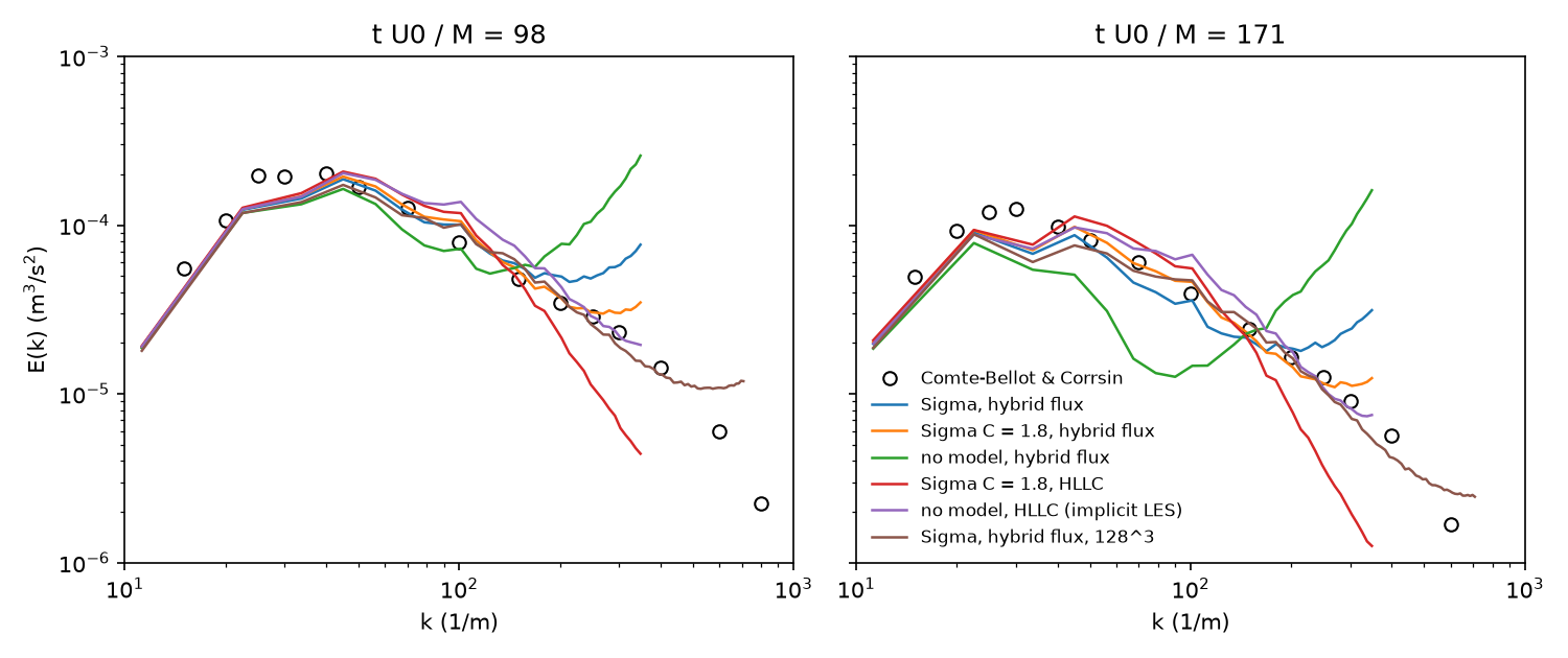
Hexahedra, MUSCL without limiter, initial phases developed by two rescaled
pre-runs. Spectral error: log10 RMS of E_LES / E_CBC for k <= 2/3 k_c;
energy: resolved energy over the measured energy up to k_c; budget:
shares of the total dissipation of resolved energy, averaged over t = 0 to
station 3 (stations 2 / 3 for the first two columns):
| Mesh | Flux | Model | Spectral error | Energy | Numerical | SGS | Molecular |
|---|---|---|---|---|---|---|---|
| 32^3 | hybrid | Sigma | 0.153 / 0.151 | 1.54 / 1.51 | -0.012 | 0.830 | 0.182 |
| 32^3 | hybrid | Sigma C = 1.8 |
0.103 / 0.082 | 1.29 / 1.20 | -0.002 | 0.891 | 0.111 |
| 64^3 | hybrid | Sigma | 0.107 / 0.104 | 1.25 / 1.02 | 0.013 | 0.691 | 0.296 |
| 64^3 | hybrid | Sigma C = 1.8 |
0.058 / 0.063 | 1.08 / 0.97 | 0.013 | 0.796 | 0.191 |
| 64^3 | hybrid | WALE | 0.090 / 0.086 | 1.20 / 0.98 | 0.007 | 0.730 | 0.263 |
| 64^3 | hybrid | Vreman | 0.108 / 0.106 | 1.25 / 1.02 | 0.012 | 0.689 | 0.298 |
| 64^3 | hybrid | Smagorinsky | 0.099 / 0.094 | 1.23 / 1.01 | 0.014 | 0.703 | 0.283 |
| 64^3 | hybrid | none | 0.226 / 0.375 | 1.81 / 1.76 | -0.077 | 0 | 1.077 |
| 64^3 | HLLC | Sigma C = 1.8 |
0.154 / 0.217 | 0.95 / 0.93 | 0.463 | 0.435 | 0.103 |
| 64^3 | HLLC | none (implicit LES) | 0.135 / 0.114 | 1.20 / 1.12 | 0.838 | 0 | 0.162 |
| 128^3 | hybrid | Sigma | 0.063 / 0.085 | 1.03 / 0.91 | 0.020 | 0.522 | 0.459 |
| 128^3 | hybrid | Sigma C = 1.8 |
0.124 / 0.141 | 0.98 / 0.92 | 0.019 | 0.651 | 0.330 |
| 128^3 | hybrid | none | 0.182 / 0.249 | 1.13 / 0.77 | 0.018 | 0 | 0.982 |
Findings:
- With the hybrid flux the model does the work: numerical dissipation
is 1-2% of the total at every resolution (
eps_num / eps_sgs <= 0.04, against the criterion 0.5). Model-off runs pile energy up atk_c(the spectrum rises by an order of magnitude) and miss the spectrum by 2-4 times the model-on error. - With HLLC everywhere the scheme does the work: 84% of the dissipation
without a model and still 46% with one (
eps_num / eps_sgs = 1.06), so such runs are implicit LES whatever the model; implicit LES matches the spectrum about as well as the explicit models at their default constants, which is why a budget, not the spectrum alone, is needed to tell them apart. - Model constant and resolution: at 64^3 (
k_cin the inertial range) every model at its literature constant leaves a pile-up over the last third of the wavenumbers; Sigma withC = 1.8matches the spectrum to 0.06 decades (15%). At 128^3 the literature constant (1.35) is the best (0.06-0.09 decades) and 1.8 over-dissipates. The second-order discretization's own transfer function acts like a larger filter on the coarser mesh. Recommendation: keepC = 1.35(the default), use 1.5-1.8 whenk_clies in the inertial range, and check with the budget and the spectrum. The channel (8.2) brackets the same range. - TENO-E with the hybrid flux (32^3) gave
eps_num = -0.22: the nonlinear stencil selection feeds energy into the resolved field when nothing upwinds it. Use MUSCL without limiter (or a linear reconstruction) with the hybrid flux; TENO stays for shocks with the Riemann flux. - The targets of this section (15% for every
k <= 2/3 k_c) are met in the mean (0.06 decades = 15%) but not point by point: the largest single-shell deviation is 31-47%, at the lowest shells (few modes, realization noise of one random field) and near2/3 k_c.
8.2 Turbulent channel flow (Moser, Kim & Mansour 1999; Lee & Moser 2015)
Re_tau = 395(and 590): box2 pi h x 2 h x pi h, periodic in x and z, isothermal no-slip walls, constant mass flow forcing at the bulk Reynolds number of the DNS (Re_b = 2 h U_b / nuabout 13,700 for 395), bulk Mach 0.2. Depends on #172 (mass-flow forcing and mesh stretching).- Mesh:
Delta x+ ~ 40-50,Delta z+ ~ 20, first celly+ < 1, tanh stretching: 64 x 64 x 64 hexahedra at 395 (96 x 96 x 96 at 590), plus a coarser48^3for refinement. - Targets: friction Reynolds number within 3% of the DNS (equivalently
C_fwithin 6%); mean velocityU+within 3% acrossy+ = 30-300; peaku'_rms+within 10% and aty+10-20;v'_rms+,w'_rms+and-<u'v'>+within 10% of their peaks. Model-off at the same mesh must missRe_tauand the peaku'_rms+by more than twice the model-on error. Budget reported per wall-normal band.
Results (stage 4, examples/channel_les)
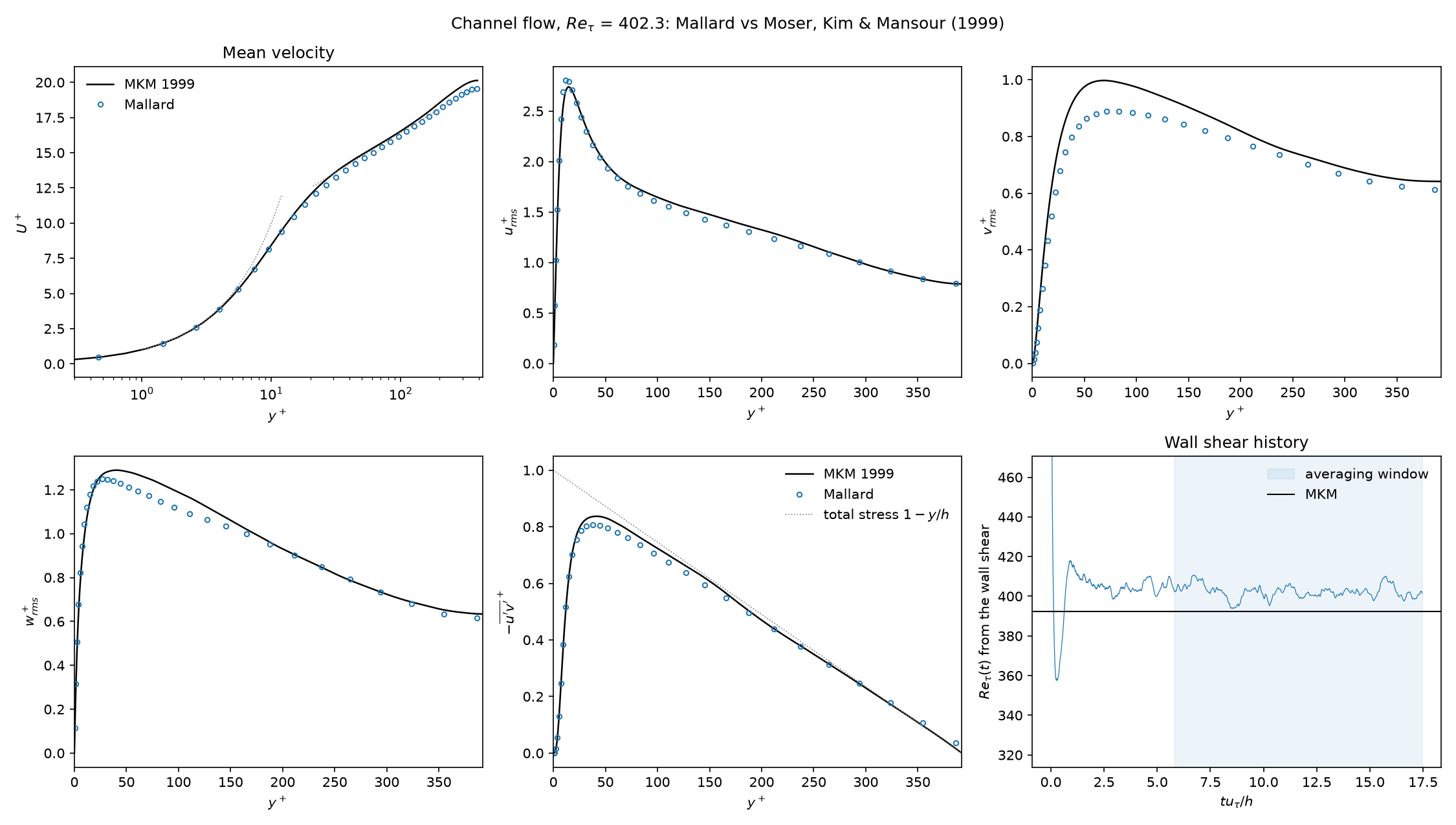
Re_tau = 395, hybrid flux, MUSCL without limiter, averaged over t =
100-300 h/U_b (11-12 h/u_tau), resolved fluctuations; dissipation shares of
the kinetic-energy budget over the same window:
| Mesh | Flux | Model | Re_tau (392.2) |
Cf |
U+(30) / U+(100) (13.49 / 16.53) |
peak v_rms+ (1.00) |
numerical / SGS / molecular |
|---|---|---|---|---|---|---|---|
| 64^3 | hybrid | Sigma | 402.3 (+2.6%) | +4.8% | 13.10 / 16.24 | 0.89 | 3.5 / 12.6 / 83.9% |
| 64^3 | hybrid | Sigma C = 1.8 |
389.4 (-0.7%) | -1.9% | 13.68 / 16.98 | 0.85 | 2.8 / 16.6 / 80.6% |
| 64^3 | hybrid | none | 420.1 (+7.1%) | +14.2% | 12.27 / 15.16 | 0.97 | 5.0 / 0 / 95.0% |
| 64^3 | HLLC | Sigma C = 1.8 |
317.6 (-19%) | -35% | 17.86 / 22.05 | 0.78 | 13.5 / 5.4 / 81.1% |
| 48^3 | hybrid | Sigma C = 1.8 |
381.3 (-2.8%) | -5.9% | 14.09 / 17.47 | 0.80 | 3.2 / 17.9 / 78.9% |
| 48^3 | hybrid | none | 405.3 (+3.3%) | +6.3% | 12.67 / 15.74 | 0.98 | 6.1 / 0 / 93.9% |
Findings:
- At 64^3 both Sigma constants meet the
Re_tautarget (3%) and the mean profile target (3% for y+ = 30-300); without a modelRe_tauis 7% high, more than twice the model-on errors.v_rms+is 11-15% low (only the resolved part is counted) and misses the 10% target;u_rms,w_rmsand-u'v'are within 10%. - At 48^3 the model-off run is closer to MKM in
Re_tauthan at 64^3 and than the model-on run at 48^3 (+3.3% against -2.8%): on this mesh the model-off result benefits from compensating errors, so the 48^3 pair does not discriminate; the 64^3 pair does. Sigma's error decreases under refinement (-2.8% -> -0.7% forC = 1.8). - The SGS model carries 13-18% of the dissipation of resolved energy; most
of it is molecular at this wall-resolved resolution. The hybrid flux's
numerical dissipation is 3-6% (
eps_num / eps_sgs= 0.17-0.28, within the criterion 0.5). - With HLLC instead of the hybrid flux the result is wrong and the budget
says why: the scheme removes 2.5 times as much resolved energy as the
model (13.5% against 5.4%), the near-wall streaks are too strong (peak
u_rms+3.77), the turbulent momentum transfer too weak, andRe_tau19% low (Cf-35%). - The DNS at
Re_tau = 180(examples/channel_retau180, 192 x 96 x 128, no model; #209), averaged over t = 80-160 h/U_b: with HLLC 6.8% of the dissipation is numerical andRe_tau = 173.7(-2.5% from MKM's 178.1, as the example's 172.6); with the hybrid flux 0.9% is numerical andRe_tau = 179.8(+0.9%). The upwind dissipation explains most of that DNS's deficit.
Results at Re_tau = 590 (examples/channel_les/input_590.toml)
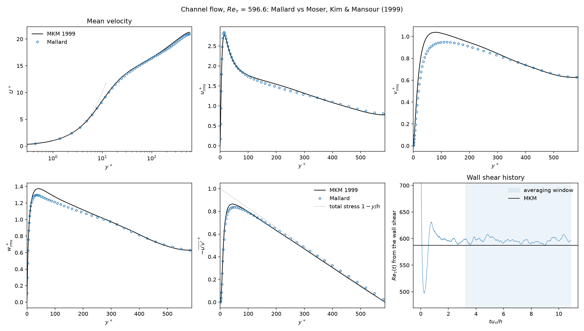
96^3 hexahedra (dx+ = 38, dz+ = 19, dy+ = 0.87 at the wall), the numerics
of the 395 case, Re_b = 21,907 (MKM's U_b+ = 18.65), averaged over t =
60-200 h/U_b (7.6-8.1 h/u_tau) after the synthetic initial field (the
figure: Sigma with Scotti's width, the default). MKM's Re_tau = 587.2:
| Model | Re_tau |
Cf |
U+(30) / U+(100) (13.53 / 16.54) |
peak u_rms+ (2.77) |
peak v_rms+ (1.04) |
numerical / SGS / molecular |
|---|---|---|---|---|---|---|
| Sigma, Scotti width (default) | 596.6 (+1.6%) | +2.9% | 13.33 / 16.43 | 2.84 | 0.95 | 3.3 / 16.2 / 80.6% |
Sigma, V^(1/3) |
611.0 (+4.1%) | +7.9% | 12.90 / 15.88 | 2.83 | 0.96 | 2.3 / 13.5 / 84.2% |
| none | 632.7 (+7.8%) | +15.7% | 12.18 / 14.92 | 2.78 | 1.02 | 3.3 / 0 / 96.7% |
- With Scotti's width the targets of this section hold at 590:
Re_tauwithin 3% (1.6%), the mean profile within 2% for y+ = 30-100,u_rms,w_rmsand-u'v'within 10%. WithV^(1/3)the model halves the model-off error but misses theRe_tautarget (+4.1%); the cells are the same in wall units as at 395, and the near-wall ones are the more anisotropic, so the width matters more.eps_num / eps_sgs= 0.20 and 0.17. v_rms+is 8-9% low at 590 and 11-12% low at 395 on 64^3 (dx+ = 39, dz+ = 19), 8% low at 395 on 96 x 64 x 96 (dx+ = 26, dz+ = 13;Re_tau396.3, +1.0%): it improves with the streamwise and spanwise resolution and barely depends on the model (Scotti 0.88,V^(1/3)0.89,C = 1.80.85, the dynamic constant 0.91, no model 0.97 at 395), so it is the resolution of the wall-normal motions of the near-wall cycle. Only the resolved part is counted; an isotropic SGS share2/3 k_sgsfrom Yoshizawa's estimate would add about 1%.
8.3 Reacting validation
- Laminar flame invariance (stage 5, H2/air and CH4/air, existing
premixed_flame): withF = 1, 4, 8,s_Lwithin 2% of the unthickened flame and of Cantera; thickness ratio within 5% ofF. - Flame-vortex or flame in decaying turbulence (2D/3D periodic box,
no inflow needed): turbulent consumption speed against the efficiency
function's prediction
E s_Lat modestu'/s_L; model-off (E = 1) comparison. - Volvo bluff-body flame (Sjunnesson, Henrikson & Löfström 1992),
propane/air
phi = 0.65, non-reacting and reacting: mean and RMS axial velocity atx/h = 0.375, 0.95, 1.53, 3.75, 9.4within 10% ofU_b, and the recirculation length. Results below: non-reacting done; reacting set up but not run at an acceptable thickening (see its plan).
Results: premixed flame in decaying turbulence (examples/flame_turbulence)
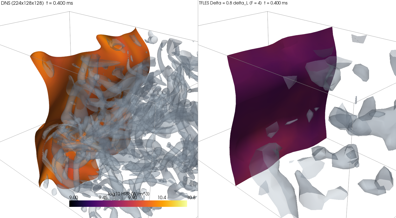
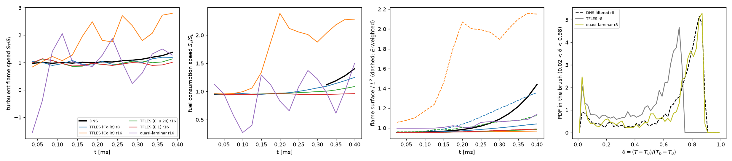
DNS reference (input.toml): stoichiometric H2/air, S_L = 2.332 m/s,
delta_L = 0.330 mm, 224 x 128 x 128 cells of delta_L / 10, u' = 2.1
S_L, l_t / delta_L = 2.4, Ka = 2.0; h / eta = 1.4, numerical
dissipation 0.4% of the total. The turbulent flame speed S_T is the rate
at which the fresh-gas volume (theta < 0.5, smooth) decreases per unit
cross-section (the fresh gas is at rest against the closed end), fitted
over the window. LES (les.toml): the same initial field box-filtered to
Delta = 4, 8, 16 DNS cells (0.40, 0.80, 1.60 delta_L; F = 2, 4, 8
at n_res = 5), domains extended on the burnt side so the thickened
burnt-gas profile is not truncated. Variants: TFLES with Colin's subgrid
velocity (the default until #294), TFLES with u' = C_u nu_t / Delta (C_u = 28),
TFLES with E = 1, quasi-laminar (Sigma model, no flame model), and no
model at all. Laminar check: the thickened laminar flames in the same
domains give S_T / S_L = 0.98-1.03.
S_T / S_L and its error against the DNS (1.132 over 0.2-0.4 ms; 1.233
over 0.3-0.4 ms, when the wrinkling has developed):
Delta / delta_L |
Colin (default until #294) | C_u = 28 |
E = 1 |
quasi-laminar | no model |
|---|---|---|---|---|---|
0.4 (F = 2) |
1.056 (-6.7%) / 1.114 (-9.7%) | 1.065 (-5.9%) / 1.126 (-8.7%) | 1.050 (-7.2%) | 1.088 (-3.9%) / 1.156 (-6.2%) | 1.086 (-4.0%) |
0.8 (F = 4) |
1.053 (-6.9%) / 1.136 (-7.9%) | 1.034 (-8.6%) / 1.082 (-12%) | 0.985 (-13%) | 1.166 (+3.0%) / 1.265 (+2.6%) | 1.164 (+2.8%) |
1.6 (F = 8) |
2.240 (+98%) / 2.361 (+91%) | 1.008 (-11%) / 1.042 (-16%) | 0.947 (-16%) | 1.051 (-7.1%) / 1.221 (-1.0%) | 1.058 (-6.6%) |
(two numbers: windows 0.2-0.4 / 0.3-0.4 ms.)
- TFLES converges to the DNS from below as
Deltadecreases and is smooth in time (rms deviation ofS_T(t)from the DNS 8-20%), with|eps_num / eps_sgs| <= 0.14(Colin r16: 0.20). The thickened flame loses most of the resolved wrinkling atF = 8(resolved surface 0.96 of the cross-section against the DNS's 1.13), soEmust supply it. - Colin's subgrid velocity overshoots at
Delta = 1.6 delta_L: meanE = 2.10andS_T+98%. The a priori test on the filtered DNS (tools/tfles_apriori.py, t = 0.125-0.2 ms, fresh gas next to the flame) shows why: Colin'su' = 2 Delta^3 |lap(curl u)|is 3.3 / 7.0 / 10S_LatDelta= 0.4 / 0.8 / 1.6delta_L, while the DNS's velocity fluctuation belowF delta_Lis 0.6 / 1.0 / 1.2S_L(5-8 times less); the wrinkling factor of the DNS's flame surface at the scaleF delta_Lis 1.003 / 1.009 / 1.022, against Colin'sE= 1.01 / 1.16 / 1.80. On coarse meshes the operator is dominated by the largest resolved eddies, which the factor 2 calibration of Colin et al. (atDeltawell inside the inertial range) does not cover. Loweringbetato 0.3 halves the overshoot (S_T1.24 atF = 8) but does not fix the operator. - Option
subgrid_velocity = "eddy_viscosity":u' = C_u nu_t / Delta. On the same filtered DNS, Mallard's Sigmanu_tgivesC_u= 22 / 28 / 39 at the three widths (a priori,Delta-dependent). Sensitivity a posteriori,S_Tover 0.2-0.4 ms:C_u= 22 / 28 / 39 gives 0.975 / 1.008 / 1.138 atF = 8and 1.013 / 1.034 / 1.101 atF = 4. It removes the overshoot, butC_uis calibrated on this DNS. - Quasi-laminar and model-off runs have the closest mean
S_Ton coarse meshes but are erratic in time (rms deviation 32-36% atDelta >= 0.8 delta_L): the flame is one or two cells thick, its speed is set by the scheme, and the numerical dissipation is 15% (quasi-laminar,F = 8;eps_num / eps_sgs= 0.39) and 21% (no model) of the total. They are not LES by the criterion of section 4.2 atDelta = 1.6 delta_L. - Temperature PDFs in the flame brush (DNS box-filtered to the LES
width): L1 distance 0.32 / 0.58 / 0.64 for TFLES, 0.04 / 0.12 / 0.33
quasi-laminar. TFLES puts the brush at intermediate temperatures, as a
thickened flame must; the unthickened flame matches the filtered DNS's
bimodal shape better at small
Delta.
Independent check (case 2), not used for any calibration: a second DNS
with a different turbulent field (seed 2, u' = 1.42 S_L, l_t = 0.75
mm, 176 x 96 x 96 cells of delta_L / 10, to 0.35 ms) and the same LES
variants. The turbulence is weaker and the flame stays nearly flat (DNS
resolved surface 0.97-1.00, S_T / S_L = 0.996 over 0.15-0.35 ms), so the
case tests whether a model invents wrinkling that is not there:
Delta / delta_L |
Colin (default until #294) | C_u = 28 |
E = 1 |
no model |
|---|---|---|---|---|
| 0.4 | 0.990 (-0.5%) | 0.991 (-0.5%) | 0.991 (-0.5%) | 0.989 (-0.6%) |
| 0.8 | 0.960 (-3.6%) | 0.974 (-2.2%) | 0.975 (-2.0%) | 0.989 (-0.7%, rms 46%) |
| 1.6 | 1.964 (+97%), E = 1.78 |
0.993 (-0.2%), E = 1.03 |
1.001 (+0.5%) | 0.930 (-6.6%, rms 47%) |
Colin's operator doubles the flame speed at Delta = 1.6 delta_L here too,
with almost no subgrid wrinkling to model; C_u = 28 stays within 4% at
every width (over 0.25-0.35 ms as well). This confirms the overshoot and
that the eddy-viscosity velocity does not add spurious wrinkling, but it
cannot validate the magnitude of C_u: E = 1 is as good in this case.
In the weak turbulence the SGS dissipation is small and eps_num is
negative (the scheme adds no dissipation of its own); eps_num <= 0.5
eps_sgs holds for every TFLES run of both cases.
Decision (#222). Colin's operator stayed the default (the published
model) and subgrid_velocity = "eddy_viscosity" (C_u = 28) became an
opt-in. Colin's efficiency overpredicts the turbulent flame speed by about
a factor of 2 at Delta = 1.6 delta_L (F = 8) in both cases, and is
within 10% for Delta <= 0.8 delta_L. C_u = 28 is calibrated a
priori on case 1 and only checked for the absence of overshoot on case 2;
S_T changes by -3% to +13% over the a priori range C_u = 22-39 (case 1, F = 8).
Superseded by the dynamic efficiency below.
Dynamic efficiency (#294)
efficiency = "dynamic" (section 6.3: E = F^beta, beta from the
flame-surface identity with a test filter of gamma = 1.51, no subgrid
velocity, no constant), on the same LES of both cases, same initial states
(case 1: the archived ones; case 2: regenerated from its HIT pre-run, seed
2 with u' = 3.4 m/s, whose LES initial kinetic energies match the
archived runs' to 1e-12). Colin's F = 8 runs were repeated on the same
build and reproduce 2.240 and 1.964.
S_T / S_L against the DNS (case 1: 1.132 over 0.2-0.4 ms / 1.233 over
0.3-0.4 ms; case 2: 0.996 over 0.15-0.35 ms / 1.000 over 0.25-0.35 ms),
with the mean E in the flame:
Case, Delta / delta_L |
dynamic | Colin | C_u = 28 |
E = 1 |
|---|---|---|---|---|
1, 0.4 (F = 2) |
1.082 (-4.4%) / 1.151 (-6.7%), E 1.03 |
-6.7% / -9.7% | -5.9% / -8.7% | -7.2% |
1, 0.8 (F = 4) |
1.068 (-5.7%) / 1.119 (-9.2%), E 1.07 |
-6.9% / -7.9% | -8.6% / -12% | -13% |
1, 1.6 (F = 8) |
1.045 (-7.7%) / 1.066 (-14%), E 1.09 |
+98% / +91% | -11% / -16% | -16% |
| 2, 0.4 | 0.996 (0.0%) / 0.996 (-0.4%), E 1.005 |
-0.5% | -0.5% | -0.5% |
| 2, 0.8 | 0.985 (-1.1%) / 0.971 (-2.9%), E 1.01 |
-3.6% | -2.2% | -2.0% |
| 2, 1.6 | 1.055 (+5.9%) / 1.107 (+11%), E 1.05 |
+97% | -0.2% | +0.5% |
- The overshoot is gone on both cases without calibration: within 8% of
the DNS at every width over the main windows (14% and 11% over the late
windows at
F = 8), against Colin's factor of 2 atF = 8. On case 1, where the flame wrinkles, it is closer to the DNS thanC_u = 28andE = 1at every width and window, and than Colin except atF = 4over the late window. On the nearly flat case 2 it adds 5-11% atF = 8, whereC_u = 28andE = 1add nothing: the remaining bias. beta(integrals columntf_beta) is 0.01-0.10 on case 1 and 0.005-0.04 on case 2, rising as the flame wrinkles;|eps_num / eps_sgs|(window means) 0.03 / 0.07 / 0.12 (case 1) and 0.38 / 0.26 / 0.46 (case 2;E = 10.37,C_u = 280.40 atF = 8).- A priori (
tools/tfles_apriori.pyon the extracted DNS snapshots: the DNS top-hat filtered atF delta_Lon the LES mesh, the model's test filter and global sums), against the wrinkling factorXiof the DNS surface at the scaleF delta_L:
| Snapshot | Xi (F = 2 / 4 / 8) |
dynamic E |
|---|---|---|
| case 1, 0.2 ms | 1.004 / 1.011 / 1.025 | 1.009 / 1.044 / 1.135 |
| case 1, 0.4 ms | 1.082 / 1.203 / 1.404 | 1.095 / 1.332 / 1.368 |
| case 2, 0.2 ms | 1.002 / 1.004 / 1.007 | 1.006 / 1.026 / 1.114 |
| case 2, 0.35 ms | 1.009 / 1.023 / 1.036 | 1.015 / 1.043 / 1.157 |
It follows the DNS's wrinkling as it grows (Colin's E at 0.125-0.2 ms:
1.01 / 1.16 / 1.80) but overpredicts by up to 11% at F = 8 when the
flame is nearly flat: Delta_e = 8 delta_L exceeds the integral scale
(l_t = 2.3-2.4 delta_L) and the test-filtered width gamma Delta_e
= 12 delta_L is that of the box (9.6-12.8 delta_L), so the surface it removes is large-scale tilt of the
front, which the power law extrapolates down to delta_L. The thickened
LES flame resolves less wrinkling than the filtered DNS, so a posteriori
E is lower (1.05-1.09 at F = 8).
- Cost (the flame_3d benchmark, 221,184 hexahedra, one A100, two runs
each): 14.7 ms per step outside the chemistry against 13.6 ms with
Colin's operator or eddy_viscosity (+8%); the chemistry's cost follows
E / F.
Decision (#294). The dynamic efficiency is the default: it removes
Colin's overshoot on both cases with no constant to calibrate and is
within 8% of the DNS at Delta = 0.4-1.6 delta_L. Colin
(efficiency = "charlette") and C_u = 28 (subgrid_velocity =
"eddy_viscosity") remain available; the Volvo input and the flame_3d
benchmark keep charlette with eddy_viscosity.
Results: non-premixed flame in decaying turbulence (PaSR, experimental)
DNS: an H2/N2 (25% H2) - air counterflow diffusion flame profile (K = 160
1/s, peak 1544 K, Z_st = 0.556) in the box and turbulence of the premixed
DNS, pressure outlets on both ends, to 0.4 ms (tools/flame_turbulence.py
init --x-f, analyze --z-fuel --z-st). LES at Delta = 0.27 and 0.53 mm
(8 and 16 DNS cells) with the Sigma model and [les.combustion] model =
"pasr", against quasi-laminar chemistry. Heat release over 0.2-0.4 ms
(DNS: stoichiometric surface 1.58, T there 1262 K):
Delta |
PaSR | quasi-laminar |
|---|---|---|
| 0.27 mm | -10.7% (kappa 0.62 at Z_st) |
+16.6% |
| 0.53 mm | -50% (T_st 892 K: near extinction; kappa 0.26) |
+41% |
eps_num / eps_sgs <= 0.10 (PaSR) and 0.23 (quasi-laminar). PaSR moves the
heat release the right way at the finer width and overcorrects at the
coarser one, where tau_mix = Delta^2 / (nu + nu_t) with C_mix = 1
overestimates the mixing time; it ships as experimental, not as a default.
Results: Volvo bluff body, non-reacting (examples/volvo_bluff_body)
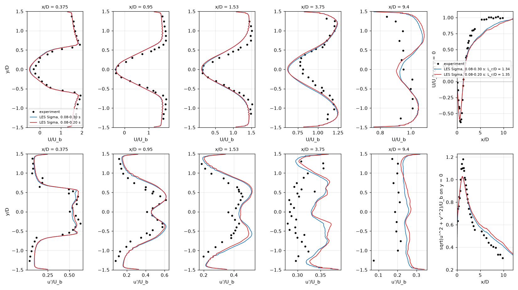
The rig of Sjunnesson et al. at the conditions of the AIAA Model Validation
for Propulsion workshop: a channel of height 3 D with an equilateral
triangle of edge D = 40 mm, air at 288 K and U_b = 16.6 m/s
(Re_D = 45,000), span periodic over 2 D (the workshop's choice; the rig
is 6 D wide), inlet 5 D upstream of the base (nscbc_inlet with
digital-filter turbulence, u' = 5% U_b, L = 10 mm), outlet 17 D
downstream (nscbc_outlet), no-slip adiabatic walls without a wall model.
Sigma with Scotti's width, hybrid flux, MUSCL without limiter, 2.7M
hexahedra (tools/make_volvo_mesh.py): Delta = 1.25 mm = D / 32 in the
near wake and shear layers, 0.6 mm at the separation corners. Statistics
over 0.08-0.30 s (about 26 shedding periods, 4 flow-throughs of the
domain), averaged over the span. Reference: the LDA data as plotted by Wu
et al. (2017), digitized from the vector figures
(examples/volvo_bluff_body/reference).
| Quantity | LES | Experiment |
|---|---|---|
Recirculation length L_r / D (mean U = 0 on the centerline) |
1.34 | 1.35 |
Centerline minimum of U / U_b (at x / D) |
-0.59 (0.61) | -0.64 (0.75) |
Mean |U - U_exp| / U_b at x/D = 0.375 / 0.95 / 1.53 / 3.75 / 9.4 |
0.13 / 0.14 / 0.11 / 0.07 / 0.08 | |
Mean |u' - u'_exp| / U_b at the same stations |
0.05 / 0.08 / 0.08 / 0.05 / 0.06 | |
Shedding frequency (Strouhal f D / U_b) |
118 Hz (0.285) | |
eps_num / eps_sgs; shares numerical / SGS / molecular |
-0.38; -52 / 135 / 17% |
- The recirculation length is within 1% and the RMS velocity within 10% of
U_bat every station. The mean axial velocity is within 10% atx/D >= 3.75but 11-14% off (mean over each profile's points) in the near wake, where the error comes from the steep shear layers and the outer flow (1.6U_bagainst 1.7 atx/D = 0.95); downstream of the bubble the centerline velocity recovers more slowly than measured (0.80 against 0.97U_batx/D = 5), which Wu et al. (2017) also report, with other solvers, for this domain and inflow. The statistics atx/D = 9.4are not converged (asymmetric). - Budget:
eps_numis negative and steady (-0.38eps_sgsin every 40 ms window from 0.08 to 0.30 s): the convective operator feeds resolved energy at 38% of the rate the model removes it, rather than dissipating it. The criterioneps_num <= 0.5 eps_sgsholds, but the sign means the model's dissipation is partly offset by the scheme, not that the scheme helps. The KEEP flux preserves kinetic energy exactly only for cell values (section 4.3); with the unlimited MUSCL states on this stretched, non-orthogonal mesh it does not, as TENO's stencil selection did not in section 8.1. The source has not been localized (the budget is a global sum). Model-off runs were not made for this case. - Mesh orthogonality matters for the central flux. A first mesh had
vertical mesh lines meeting the slanted faces at 60 degrees: the wall
cells there grew grid-scale velocity up to Mach 0.4-0.8 within 15-40 ms
(also with
upwind_floor = 0.05), while the same flow with HLLC stayed below 0.15. With mesh lines normal to the faces the largest Mach number stays at 0.2 (the separation corners). A non-rectangular inlet block (curved mesh lines up to the inlet face) diverged in 230 steps; the inlet half of the upstream block is now Cartesian. - Cost: 626,000 steps of 0.48 us (acoustic CFL 0.8 at the 0.54 mm wall cells), 14 ms each on four A100s (2.8 hours).
Volvo bluff body, reacting: set up, not validated
examples/volvo_bluff_body/reacting.toml: propane-air at phi = 0.65, 288
K, U_b = 17.3 m/s; mechanisms/c3h8_2step.yaml, the two-step mechanism of
Westbrook & Dryer (1981) with its fuel step tuned to GRI-Mech 3.0's laminar
flame (s_L 0.209 m/s as GRI, T_b 1766 K against 1792, thermal thickness
0.471 mm against 0.552; Mallard's 1D flame on it: s_L -1.5%, T_max 1767
K, thickness 0.473 mm). TFLES with the eddy-viscosity efficiency.
What a first attempt on a 2 mm mesh (0.66M cells, F = 21) showed before
it was stopped:
- Cost: 85 ms per step on four A100s, 8M cells/s, about 24 times the
cost per cell of the non-reacting flow (chemistry about 40% of it); unity
Lewis numbers saved nothing and looser integrator tolerances (
rtol1e-5,atol1e-8) made the chemistry five times slower. - Ignition: burnt gas only in the wake was flushed out before the recirculation zone formed, and the flame blew off. Burnt gas filling the channel downstream of the base works, but the fresh/burnt contact the inflow then pushes out overshoots under the central flux (2550 K from a 2 mm edge, 1890 K from an 8 mm one); double flux diverged within 700-2800 steps.
Thickening must stay at F <= 5, i.e. Delta <= delta_L = 0.47 mm
wherever the flame is, with n_res = 5. Estimated cost (0.20 s simulated:
0.06 s to establish the flame, 0.14 s of statistics; acoustic time step
proportional to the smallest cell; 2M cells/s per A100):
| Mesh | Cells | F |
Steps | Time on A100s | GPU hours |
|---|---|---|---|---|---|
| 2 mm | 0.66M | 21 | 470k | 11 h on 4 | 45 |
| 1.25 mm (the non-reacting mesh) | 2.7M | 13 | 800k | 19 h on 16 | 300 |
| 1.0 mm | 5.3M | 11 | 1.0M | 31 h on 24 | 740 |
| 0.47 mm in the flame region (x < 10 D), coarser elsewhere, span 2 D | ~28M | 5 | 1.3M | ~220 h on 24 | ~5,000 |
| the same, span 1 D | ~15M | 5 | 1.3M | ~120 h on 24 | ~2,700 |
The F <= 5 case is out of reach until the mixture solver is faster per
cell; the two-step mechanism is already the smallest that gives s_L
and T_b, so chemistry is not the lever. The affordable reacting test of
the inflow-outflow path at F <= 5 is a premixed slot (Bunsen) jet with
digital-filter inflow, LES against a Mallard DNS of the same case, as
for the flame in decaying turbulence.
9. Stages
One pull request each, stacked; the umbrella issue links them.
- SGS eddy viscosity:
[les]with Sigma, WALE, Vreman, Smagorinsky; filter width; SGS heat and species fluxes (single gas and mixtures); time step;MU_T; dissipation budget in[integrals]; tests and docs. - Hybrid convective flux: KEEP flux and compression-only Ducros sensor for single gases, mixtures and double flux; tests and docs.
- Decaying isotropic turbulence validation (Comte-Bellot & Corrsin): initial-field tool, reference data, example, budget study (upwind vs hybrid, model on vs off, 32^3/64^3).
- Channel validation at
Re_tau = 395(590 if affordable), after #172. - TFLES: thickening, sensor, Charlette efficiency with Colin's operator, per-cell chemistry time scaling; laminar-flame invariance tests.
- Reacting validation: flame in decaying turbulence, Volvo bluff body.
- Optional: PaSR; dynamic Sigma / Lagrangian dynamic Smagorinsky; Scotti filter width; AMD.
10. Risks
- Hybrid flux stability on irregular tetrahedral meshes. Mitigation:
phi_min, tests on tetrahedra, budget. - Sigma's closed-form singular values lose relative accuracy for
nearly degenerate
Gin single precision. Mitigation: evaluated in double in every build, clipped to non-negative eigenvalues. - The budget's
Piis only as accurate as the gradients; reported with the result and small in the target cases. - Channel cost at
Re_tau = 590(about 1M cells,10^5steps): one A100 for about a day; 395 first. - TFLES sensor based on temperature misses flames with strong heat loss; the reaction-rate sensor is the documented alternative.
References
DOIs checked against Crossref. Entries move to references.md with the stage that implements them.
- Bhagatwala & Lele 2009, J. Comput. Phys. 228, 4965. doi:10.1016/j.jcp.2009.04.009
- Butler & O'Rourke 1977, Proc. Combust. Inst. 16, 1503. doi:10.1016/S0082-0784(77)80432-3
- Charlette, Meneveau & Veynante 2002, Combust. Flame 131, 159. doi:10.1016/S0010-2180(02)00400-5
- Colin, Ducros, Veynante & Poinsot 2000, Phys. Fluids 12, 1843. doi:10.1063/1.870436
- Comte-Bellot & Corrsin 1971, J. Fluid Mech. 48, 273. doi:10.1017/S0022112071001599
- Deardorff 1970, J. Fluid Mech. 41, 453. doi:10.1017/S0022112070000691
- Ducros, Ferrand, Nicoud, Weber, Darracq, Gacherieu & Poinsot 1999, J. Comput. Phys. 152, 517. doi:10.1006/jcph.1999.6238
- Erlebacher, Hussaini, Speziale & Zang 1992, J. Fluid Mech. 238, 155. doi:10.1017/S0022112092001678
- Filatyev, Driscoll, Carter & Donbar 2005, Combust. Flame 141, 1. doi:10.1016/j.combustflame.2004.07.010
- Garnier, Adams & Sagaut 2009, Large Eddy Simulation for Compressible Flows, Springer. doi:10.1007/978-90-481-2819-8
- Garnier, Mossi, Sagaut, Comte & Deville 1999, J. Comput. Phys. 153, 273. doi:10.1006/jcph.1999.6268
- Germano, Piomelli, Moin & Cabot 1991, Phys. Fluids A 3, 1760. doi:10.1063/1.857955
- Ghosal 1996, J. Comput. Phys. 125, 187. doi:10.1006/jcph.1996.0088
- Haselbacher & Vasilyev 2003, J. Comput. Phys. 187, 197. doi:10.1016/S0021-9991(03)00095-0
- Jameson 2008, J. Sci. Comput. 34, 188. doi:10.1007/s10915-007-9172-6
- Kuya, Totani & Kawai 2018, J. Comput. Phys. 375, 823. doi:10.1016/j.jcp.2018.08.058
- Lee & Moser 2015, J. Fluid Mech. 774, 395. doi:10.1017/jfm.2015.268
- Légier, Poinsot, Varoquié, Lacas & Veynante 2002, in Advances in LES of Complex Flows, Springer, 315. doi:10.1007/978-94-017-1998-8_27
- Lilly 1992, Phys. Fluids A 4, 633. doi:10.1063/1.858280
- Meneveau, Lund & Cabot 1996, J. Fluid Mech. 319, 353. doi:10.1017/S0022112096007379
- Mittal & Moin 1997, AIAA J. 35, 1415. doi:10.2514/2.253
- Moin, Squires, Cabot & Lee 1991, Phys. Fluids A 3, 2746. doi:10.1063/1.858164
- Moser, Kim & Mansour 1999, Phys. Fluids 11, 943. doi:10.1063/1.869966
- Najafi-Yazdi, Najafi-Yazdi & Mongeau 2015, J. Comput. Phys. 292, 272. doi:10.1016/j.jcp.2015.03.034
- Nicoud & Ducros 1999, Flow Turbul. Combust. 62, 183. doi:10.1023/A:1009995426001
- Nicoud, Baya Toda, Cabrit, Bose & Lee 2011, Phys. Fluids 23, 085106. doi:10.1063/1.3623274
- Poinsot & Veynante 2012, Theoretical and Numerical Combustion, 3rd ed., self-published.
- Rozema, Bae, Moin & Verstappen 2015, Phys. Fluids 27, 085107. doi:10.1063/1.4928700
- Sabelnikov & Fureby 2013, Combust. Flame 160, 83. doi:10.1016/j.combustflame.2012.09.008
- Scotti, Meneveau & Lilly 1993, Phys. Fluids A 5, 2306. doi:10.1063/1.858537
- Sjunnesson, Henrikson & Löfström 1992, AIAA Paper 92-3650. doi:10.2514/6.1992-3650
- Smagorinsky 1963, Mon. Weather Rev. 91, 99. doi:10.1175/1520-0493(1963)091<0099:GCEWTP>2.3.CO;2
- Vreman 2004, Phys. Fluids 16, 3670. doi:10.1063/1.1785131
- Vreman, Geurts & Kuerten 1995, Appl. Sci. Res. 54, 191. doi:10.1007/BF00849116
- Wang, Boileau & Veynante 2011, Combust. Flame 158, 2199. doi:10.1016/j.combustflame.2011.04.008
- Westbrook & Dryer 1981, Combust. Sci. Technol. 27, 31. doi:10.1080/00102208108946970
- Wu, Ma, Lv & Ihme 2017, AIAA Paper 2017-1573 (arXiv:1707.05805). doi:10.2514/6.2017-1573