Documentation of the main branch

These pages follow Mallard's main branch, which is ahead of release 0.8.0: some features they describe come with the next release.

Numerical fluxes

This chapter gives the numerical flux \(\hat{\mathbf{F}}\) of eq. (2) of chapter 5: the approximate Riemann solvers, the hybrid central-upwind flux of large-eddy simulation, their extension to gas mixtures, the species fluxes, and the discrete viscous and diffusive fluxes. Face states come from chapter 5. Usage: Numerics; the carbuncle and stationary-shock studies: Numerical methods.

All solvers take the reconstructed states as \(\mathbf{W} = [\rho, \mathbf{u}, p]\) on each side and a unit normal \(\mathbf{n}\) from left to right, and return the flux per unit area (src/numerics/riemann_solver.h). With \(u_n = \mathbf{u}\cdot\mathbf{n}\) and the physical flux

\[ \begin{equation} \mathbf{F}_n(\mathbf{W}) = \left[\rho u_n,\ \rho\mathbf{u}\,u_n + p\,\mathbf{n},\ (\rho E + p)\,u_n\right]^T, \label{eq:physical-flux} \end{equation} \]

a single gas has \(\rho E = p/(\gamma - 1) + \tfrac12\rho\lvert\mathbf{u}\rvert^2\) and \(a = \sqrt{\gamma p/\rho}\); mixtures use each side's frozen pair, eq. (5) of chapter 2 (below).

Riemann solvers

[numerics] riemann_solver selects one of the following.

Rusanov

(Rusanov 1962)

\[ \begin{equation} \hat{\mathbf{F}} = \tfrac12\left(\mathbf{F}_n^L + \mathbf{F}_n^R\right) - \tfrac12 S_{\max}\left(\mathbf{U}^R - \mathbf{U}^L\right), \qquad S_{\max} = \max\left(\lvert u_n^L\rvert + a^L,\ \lvert u_n^R\rvert + a^R\right). \label{eq:rusanov} \end{equation} \]

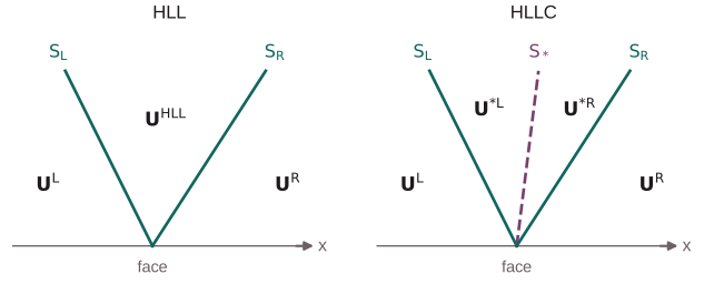
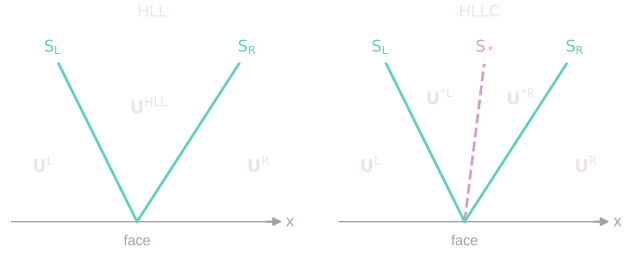
HLL

(Harten, Lax & van Leer 1983) with the wave-speed estimates of Einfeldt from Roe averages (Einfeldt 1988; Einfeldt et al. 1991):

\[ \begin{equation} \hat{\mathbf{F}} = \begin{cases} \mathbf{F}_n^L & 0 \le S_L, \\ \mathbf{F}_n^R & S_R \le 0, \\ \dfrac{S_R\mathbf{F}_n^L - S_L\mathbf{F}_n^R + S_L S_R\left(\mathbf{U}^R - \mathbf{U}^L\right)}{S_R - S_L} & \text{otherwise}, \end{cases} \qquad \begin{aligned} S_L &= \min\left(u_n^L - a^L,\ \tilde u_n - \tilde a\right), \\ S_R &= \max\left(u_n^R + a^R,\ \tilde u_n + \tilde a\right), \end{aligned} \label{eq:hll-1} \end{equation} \]

where, with the weights \(\omega_{L,R} = \sqrt{\rho^{L,R}}/(\sqrt{\rho^L} + \sqrt{\rho^R})\),

\[ \begin{equation} \tilde{\mathbf{u}} = \omega_L\mathbf{u}^L + \omega_R\mathbf{u}^R, \qquad \tilde H = \omega_L H^L + \omega_R H^R, \qquad \tilde a^2 = \max\left(0,\ (\gamma - 1)\left(\tilde H - \tfrac12\lvert\tilde{\mathbf{u}}\rvert^2\right)\right). \label{eq:hll-2} \end{equation} \]

HLLC

(Toro, Spruce & Speares 1994; Toro 2009, eqs. 10.37-10.39) with the same \(S_L\), \(S_R\). Between them, the contact speed

\[ \begin{equation} S_\star = \frac{p^R - p^L + \rho^L u_n^L(S_L - u_n^L) - \rho^R u_n^R(S_R - u_n^R)}{\rho^L(S_L - u_n^L) - \rho^R(S_R - u_n^R)} \label{eq:hllc-1} \end{equation} \]

selects the side \(K = L\) if \(S_\star \ge 0\), else \(K = R\), and

\[ \begin{equation} \hat{\mathbf{F}} = \mathbf{F}_n^K + S_K\left(\mathbf{U}^{\star K} - \mathbf{U}^K\right), \qquad \mathbf{U}^{\star K} = \rho^K\frac{S_K - u_n^K}{S_K - S_\star} \begin{bmatrix} 1 \\ \mathbf{u}^K + (S_\star - u_n^K)\,\mathbf{n} \\ E^K + (S_\star - u_n^K)\left(S_\star + \dfrac{p^K}{\rho^K(S_K - u_n^K)}\right) \end{bmatrix}. \label{eq:hllc-2} \end{equation} \]

HLLC is the default solver.

Roe

(Roe 1981) with Harten's entropy fix on the acoustic waves (Harten 1983):

\[ \begin{equation} \hat{\mathbf{F}} = \tfrac12\left(\mathbf{F}_n^L + \mathbf{F}_n^R\right) - \tfrac12\sum_k \lvert\tilde\lambda_k\rvert^{\ast}\,\alpha_k\,\tilde{\mathbf{r}}_k, \qquad \alpha_k = \tilde{\mathbf{l}}_k\cdot\left(\mathbf{U}^R - \mathbf{U}^L\right), \label{eq:roe-1} \end{equation} \]

with the eigenvalues \(\tilde u_n - \tilde a\), \(\tilde u_n\) (entropy and \(d - 1\) shear waves) and \(\tilde u_n + \tilde a\) and the left and right eigenvectors of the Euler flux Jacobian in direction \(\mathbf{n}\) at the Roe average eq. \(\eqref{eq:hll-2}\) with \(\tilde\rho = \sqrt{\rho^L\rho^R}\) (\(\tilde a^2\) floored at \(10^{-14}\)). For the two acoustic waves,

\[ \begin{equation} \lvert\lambda\rvert^{\ast} = \begin{cases} \lvert\lambda\rvert & \lvert\lambda\rvert \ge \delta, \\ \dfrac{\lambda^2 + \delta^2}{2\delta} & \lvert\lambda\rvert < \delta, \end{cases} \qquad \delta = 0.1\,\tilde a. \label{eq:roe-2} \end{equation} \]

RHLL

The rotated hybrid of Nishikawa & Kitamura 2008 applies HLL along the direction of the velocity jump, normal to shocks where Roe's lack of dissipation grows carbuncles, and Roe across it, where it keeps shear layers and contacts sharp:

\[ \begin{equation} \mathbf{n}_1 = \pm\frac{\Delta\mathbf{u}}{\lvert\Delta\mathbf{u}\rvert}, \quad \alpha_1 = \mathbf{n}_1\cdot\mathbf{n} \ge 0, \qquad \mathbf{n}_2 = \frac{\mathbf{n} - \alpha_1\mathbf{n}_1}{\lvert\mathbf{n} - \alpha_1\mathbf{n}_1\rvert}, \quad \alpha_2 = \lvert\mathbf{n} - \alpha_1\mathbf{n}_1\rvert, \label{eq:rhll-1} \end{equation} \]

\[ \begin{equation} \hat{\mathbf{F}}_\mathrm{rot} = \alpha_1\,\hat{\mathbf{F}}_\mathrm{HLL}(\mathbf{n}_1) + \alpha_2\,\hat{\mathbf{F}}_\mathrm{Roe}(\mathbf{n}_2), \label{eq:rhll-2} \end{equation} \]

with \(\Delta\mathbf{u} = \mathbf{u}^R - \mathbf{u}^L\), the sign of \(\mathbf{n}_1\) chosen so that \(\alpha_1 \ge 0\), and \(\alpha_1^2 + \alpha_2^2 = 1\). If \(\lvert\Delta\mathbf{u}\rvert \le 10^{-12}\,a_\mathrm{ref}\), with \(a_\mathrm{ref} = \max(a^L, a^R)\), then \(\mathbf{n}_1 = \mathbf{n}\) and the flux is HLL; the Roe term is dropped where \(\alpha_2\) vanishes. On tetrahedra the rotation turns HLL toward the shock normal on every face that crosses a shock, which grows a carbuncle on the stagnation line of blunt bodies, so Mallard blends the rotated flux toward HLL along the face normal by the pressure jump across the face, with the pressure weight of the AUSMPW+ scheme (Kim, Kim & Rho 2001):

\[ \begin{equation} \hat{\mathbf{F}}_\mathrm{RHLL} = w\,\hat{\mathbf{F}}_\mathrm{rot} + (1 - w)\,\hat{\mathbf{F}}_\mathrm{HLL}(\mathbf{n}), \qquad w = \min\left(\frac{p^L}{p^R}, \frac{p^R}{p^L}\right)^3. \label{eq:rhll-3} \end{equation} \]

Contacts and shear layers carry no pressure jump (\(w = 1\)) and keep the rotated flux. Only this weight comes from AUSMPW+; Mallard has no AUSM-family flux.

Hybrid central-upwind flux

[numerics] convective_flux = "hybrid", meant for large-eddy simulation, blends a non-dissipative central flux with the Riemann solver (src/numerics/flux_functor.h). The central flux is the kinetic-energy- and entropy-preserving (KEEP) flux of Kuya, Totani & Kawai 2018 with arithmetic means \(\lbrace \phi\rbrace = \tfrac12(\phi^L + \phi^R)\):

\[ \begin{equation} \hat{\mathbf{F}}_\mathrm{KEEP} = \begin{bmatrix} C \\ C\,\lbrace \mathbf{u}\rbrace + \lbrace p\rbrace \,\mathbf{n} \\ C\left(\lbrace e\rbrace + \tfrac12\,\mathbf{u}^L\cdot\mathbf{u}^R\right) + \tfrac12\left(p^L u_n^R + p^R u_n^L\right) \end{bmatrix}, \qquad C = \lbrace \rho\rbrace \,\lbrace \mathbf{u}\rbrace \cdot\mathbf{n}. \label{eq:hybrid-central-upwind-flux-1} \end{equation} \]

Its momentum flux has Jameson's form, so with cell values on both sides the convective fluxes change the kinetic energy only through the pressure work \(\lbrace p\rbrace (u_n^R - u_n^L)\) per face. The upwind fraction of each cell comes from the Ducros sensor restricted to compressions (Ducros et al. 1999; Bhagatwala & Lele 2009), evaluated at every stage from the viscous cell gradients (chapter 5):

\[ \begin{equation} \phi_i = \begin{cases} 1 & \nabla\cdot\mathbf{u} < 0 \ \text{and}\ (\nabla\cdot\mathbf{u})^2 > \theta_D\left((\nabla\cdot\mathbf{u})^2 + \lvert\nabla\times\mathbf{u}\rvert^2\right), \\ \phi_\mathrm{floor} & \text{otherwise}, \end{cases} \label{eq:hybrid-central-upwind-flux-2} \end{equation} \]

with \(\theta_D\) = [numerics.hybrid] sensor_threshold (default 0.65) and \(\phi_\mathrm{floor}\) = upwind_floor (default 0). A face takes the larger fraction of its two cells, \(\phi_f = \max(\phi_L, \phi_R)\); boundary faces take 1, except walls and symmetry planes, whose mirror states make the central flux exact and which take their cell's. At every face point,

\[ \begin{equation} \hat{\mathbf{F}} = \hat{\mathbf{F}}_\mathrm{KEEP} + \phi_f\left(\hat{\mathbf{F}}_\mathrm{Riemann} - \hat{\mathbf{F}}_\mathrm{KEEP}\right), \label{eq:hybrid-central-upwind-flux-3} \end{equation} \]

where the low-Mach correction (eq. (14) of chapter 5) applies to the Riemann flux only. The hybrid flux is not available with SIMPLER splitting (chapter 3). Its validation: LES design notes.

Gas mixtures

For mixtures each side carries its frozen pair \((\gamma, e_0)\) of eq. (5) of chapter 2, reconstructed to the face (chapter 5), and the physical flux uses \(\rho E = p/(\gamma - 1) + \rho e_0 + \tfrac12\rho\lvert\mathbf{u}\rvert^2\) on that side (riemann::SideThermo):

• Wave speeds (HLL, HLLC, RHLL) use each side's \(a = \sqrt{\gamma p/\rho}\) and the Roe average of eq. \(\eqref{eq:hll-2}\) with \(\sqrt{\rho}\)-weighted \(\tilde\gamma\), \(\tilde e_0\) and \(\tilde a^2 = (\tilde\gamma - 1)(\tilde H - \tilde e_0 - \tfrac12\lvert\tilde{\mathbf{u}}\rvert^2)\), equal to the single-gas estimate when both sides share \(\gamma\) and \(e_0 = 0\). The HLLC star states \(\eqref{eq:hllc-2}\) hold for any equation of state.

• Roe (Glaister 1988; Shuen, Liou & van Leer 1990) is written in jump form. The entropy, shear and composition waves all move at \(\tilde u_n\), so together they carry whatever part of \(\Delta\mathbf{U}\) the acoustic waves leave:

  \[ \begin{equation} \hat{\mathbf{F}} = \tfrac12\left(\mathbf{F}_n^L + \mathbf{F}_n^R - \lvert\tilde u_n\rvert\,\Delta\mathbf{U} - \sum_\pm\left(\lvert\tilde u_n \pm \tilde a\rvert^{\ast} - \lvert\tilde u_n\rvert\right)\frac{\Delta p \pm \tilde\rho\tilde a\,\Delta u_n}{2\tilde a^2} \begin{bmatrix}1 \\ \tilde{\mathbf{u}} \pm \tilde a\,\mathbf{n} \\ \tilde H \pm \tilde a\,\tilde u_n\end{bmatrix}\right), \label{eq:gas-mixtures} \end{equation} \]

  exact at contacts between different gases for any averaged sound speed, and equal to the single-gas Roe solver for one gas. - Rusanov and KEEP use each side's own \(a\) and \(e = p/((\gamma - 1)\rho) + e_0\). - The low-Mach correction uses each side's own \(\gamma\) in its Mach number.

With double flux, each face evaluates these fluxes twice, with each cell's frozen pair on both sides, as chapter 2 describes.

Species fluxes

The partial densities are transported by mass-flux upwinding (Larrouturou 1991; SpeciesSlotFunctor, src/numerics/mixture_flux.h): with \(\dot m_q\) the mass component of \(\hat{\mathbf{F}}\) at face point \(q\) (positive from left to right; the mean of the two fluxes with double flux),

\[ \begin{equation} \hat F_{\rho Y_k, q} = \max(\dot m_q, 0)\,Y_{k,q}^L + \min(\dot m_q, 0)\,Y_{k,q}^R, \label{eq:species-fluxes} \end{equation} \]

with \(Y_{k,q}^{L,R}\) the reconstructed face mass fractions of each side (chapter 5). Each cell writes the mass of every species leaving it through each of its faces, so no two threads write the same entry. On boundary faces the inflowing mass fractions are the prescribed ones (nscbc_inlet, upt), those of the image face or image cell of transmissive boundaries, or the interior ones. Since the face mass fractions lie in \([0, 1]\) and sum to one, the species fluxes sum to the mass flux, and \(\rho Y_k\) stays non-negative under the flow's CFL limit.

Viscous fluxes

The viscous fluxes use one point per face, at its centroid (ViscousFluxFunctor, src/numerics/viscous_flux.h; MixtureViscousFluxFunctor, src/numerics/mixture_viscous_flux.h).

Face values and gradients

For a variable \(q\) (velocity components, \(T\), and for mixtures \(X_k\)) on an interior face between cells \(L\) and \(R\), with \(\mathbf{d} = \mathbf{x}_R - \mathbf{x}_L\) (across periodic faces, \(R\) at its translated position),

\[ \begin{equation} q_f = \tfrac12(q_L + q_R), \qquad \nabla q_f = \overline{\nabla q} + \frac{(q_R - q_L) - \overline{\nabla q}\cdot\mathbf{d}}{\mathbf{d}\cdot\mathbf{n}}\,\mathbf{n}, \qquad \overline{\nabla q} = \tfrac12\left(\nabla q_L + \nabla q_R\right), \label{eq:face-values-and-gradients} \end{equation} \]

the average of the cell gradients of chapter 5 corrected along the face normal so that its component along the line of centroids equals the direct difference (Diskin et al. 2010). This suppresses odd-even decoupling and stays consistent on non-orthogonal meshes. Axisymmetric runs interpolate to the face center's projection on the line of centroids, and subtract from \(q_R - q_L\) the part of the jump of two r-weighted averages due to the cells' different spreads.

Boundary faces:

• walls: a one-sided difference between the cell centroid and the wall replaces the normal component of the cell gradient, \(\nabla q_f = \nabla q_i + \left((q_w - q_i)/d - \nabla q_i\cdot\mathbf{n}\right)\mathbf{n}\), with \(q_w\) the wall velocity, the wall temperature of isothermal walls, and \(d\) the normal distance from the centroid to the face. Adiabatic walls carry no heat flux and heat-flux walls the prescribed one;
• symmetry planes: only the normal stress, no work (the normal velocity vanishes), no heat or species flux;
• transmissive faces with an image face (chapter 8): the values and gradients of that interior face, eq. \(\eqref{eq:face-values-and-gradients}\);
• outflow, far-field and characteristic faces (and transmissive faces without an image): the cell's values with the normal derivatives removed;
• mixture upt faces: the cell's values and gradients.

Single gas

With \(\mu = \mu(T_f)\) from eq. (6) of chapter 1 and \(\lambda = \mu c_p/Pr\) at the face temperature (plus \(\mu_t\), \(\lambda_t\) averaged from the two cells in LES, none at walls),

\[ \begin{equation} \mathbf{F}^v_f = A_f\left[0,\ \boldsymbol{\tau}_f\cdot\mathbf{n},\ \mathbf{u}_f\cdot(\boldsymbol{\tau}_f\cdot\mathbf{n}) + \lambda\,\nabla T_f\cdot\mathbf{n}\right]^T, \label{eq:single-gas} \end{equation} \]

with \(\boldsymbol{\tau}_f\) from eq. (5) of chapter 1 at the face gradients (with the hoop term \(u_r/r\) in the divergence for axisymmetric runs) and \(\nabla T = (\nabla p - RT\nabla\rho)/(\rho R)\) from the gradients of \(\mathbf{W}\).

Mixture diffusive fluxes

The transport coefficients \(\mu\), \(\lambda\), \(\rho D_k W_k/\overline{W}\) and \(D_k^T\) are computed per cell (eqs. (7)-(13) of chapter 2) and averaged to the face. With \(c_k = \overline{\rho D_k W_k/\overline{W}}\) on the face and \(Y_{k,f}\) the face average of the cell mass fractions, eq. (10) of chapter 2 becomes

\[ \begin{equation} j_{k,f} = -c_k\,\frac{\partial X_k}{\partial n} + \frac{Y_{k,f}}{\sum_j Y_{j,f}}\sum_j c_j\,\frac{\partial X_j}{\partial n} - D^T_{k,f}\,\frac{1}{T_f}\frac{\partial T}{\partial n}, \label{eq:mixture-diffusive-fluxes} \end{equation} \]

so \(\sum_k j_{k,f} = 0\) to round-off, and the energy flux carries \(\sum_k h_k(T_f)\,j_{k,f}\) besides the work of the stress and the conduction. In LES, \(c_k\) gains \(\mu_t W_k/(Sc_t\overline{W})\). Walls and symmetry planes carry no heat or species flux (adiabatic, non-catalytic walls).