Documentation of the main branch

These pages follow Mallard's main branch, which is ahead of release 0.8.0: some features they describe come with the next release.

Boundary conditions and sources¶

This chapter gives the exterior states through which every boundary condition acts, the characteristic (NSCBC) boundaries, and the source terms \(\mathbf{S}\) of eq. (3) of chapter 1. Usage: Boundary conditions and Sources and sponges; design: characteristic boundaries, periodic boundaries.

Weak imposition¶

Every boundary condition is imposed weakly: a boundary face's convective flux is the Riemann solver applied to the interior face state \(\mathbf{W}^L\) and an exterior state \(\mathbf{W}^b\) (BoundaryData::exterior_W, src/boundary/boundary.h), with the unit normal \(\mathbf{n}\) pointing out of the domain. Ghost states also feed the least-squares gradients (chapter 5) and the mirror images of TENO-E stencils. The viscous fluxes of each boundary type are in chapter 6. With \(u_n = \mathbf{u}^L\cdot\mathbf{n}\), the exterior states \(\mathbf{W}^b = [\rho, \mathbf{u}, p]^b\) are:

symmetry, inviscid walls: \([\rho^L,\ \mathbf{u}^L - 2u_n\mathbf{n},\ p^L]\);
wall_adiabatic, wall_heat_flux (viscous): \([\rho^L,\ 2\mathbf{u}_w - \mathbf{u}^L,\ p^L]\);
wall_isothermal (viscous, single gas): as above, with \(\rho^b = p^L/(R\,T^b)\), \(T^b = \max(2T_w - T^L,\ 0.1\,T_w)\);
upt, dirichlet: the prescribed state (dirichlet: per face, from expressions);
farfield: eq. \(\eqref{eq:far-field}\);
p_out: subsonic (\(u_n < a^L\)): \([\rho^L p_b/p^L,\ \mathbf{u}^L,\ p_b]\), keeping \(T\); supersonic: \(\mathbf{W}^L\);
p_out_average: as p_out with \(p^L + \Delta p\), \(\Delta p\) the target minus the area average of the adjacent cells' pressure, updated at every stage (and \(p \ge 10^{-3}p^L\));
extrapolation: the image-face state, below;
nscbc_outlet, nscbc_inlet: eq. \(\eqref{eq:characteristic-boundaries-3}\).

\(\mathbf{u}_w\) is the wall velocity and \(T_w\) the wall temperature. Under gravity, walls and symmetry planes continue the hydrostatic pressure in their ghosts: a ghost at distance \(\delta\) beyond the face has \(p^b = p^L + \rho^L(\mathbf{g}\cdot\mathbf{n})\,\delta\). For gas mixtures the exterior state also carries the mass fractions and \((\gamma, e_0)\): the prescribed ones at upt faces, the image's at transmissive faces, the interior's elsewhere. Walls are adiabatic and non-catalytic for mixtures (wall_isothermal is not available).

Far field¶

The characteristic far field (Blazek 2015) takes the outgoing Riemann invariant from the interior and the incoming one from the free stream \(\mathbf{W}_\infty\):

\[ \begin{equation} \begin{aligned} R^{+} &= u_n + \frac{2a^L}{\gamma - 1}, \qquad R^{-} = u_{n,\infty} - \frac{2a_\infty}{\gamma - 1}, \qquad u_n^b = \tfrac12\left(R^+ + R^-\right), \qquad a^b = \tfrac{\gamma - 1}{4}\left(R^+ - R^-\right), \\ s &= p/\rho^\gamma \text{ and } \mathbf{u} - u_n\mathbf{n} \text{ from the upwind side}\ (\infty \text{ if } u_n^b < 0), \qquad \rho^b = \left(\frac{(a^b)^2}{\gamma s}\right)^{1/(\gamma - 1)}, \qquad p^b = \rho^b (a^b)^2/\gamma. \end{aligned} \label{eq:far-field} \end{equation} \]

Supersonic faces take \(\mathbf{W}_\infty\) at inflow and \(\mathbf{W}^L\) at outflow.

Transmissive boundaries¶

extrapolation faces, and characteristic faces before their characteristic treatment, take the state of an image face: the interior face reached by translating the boundary face inward by the depth of the boundary cell, with its reconstructed state on the far side at the matching quadrature point; without one, the state of the image cell, else the interior state. This is exactly what an interior face sees for a solution that does not vary normal to the boundary, at any order. A zero-gradient copy of the boundary cell would feed the cell back to itself at inflow boundaries, and on triangles, whose centroids are offset from the face, create an O(1) mass imbalance at moving shocks.

Periodic boundaries¶

Periodic zone pairs are joined into interior faces whose second cell is translated next to the first (src/mesh/periodic.cpp), so every scheme treats the seam as interior.

Walls¶

The ghost states above, together with the viscous wall fluxes of chapter 6, give no-slip walls with one-sided wall gradients. In LES the wall faces carry the molecular fluxes only, with no SGS stress, heat or species flux.

Characteristic boundaries¶

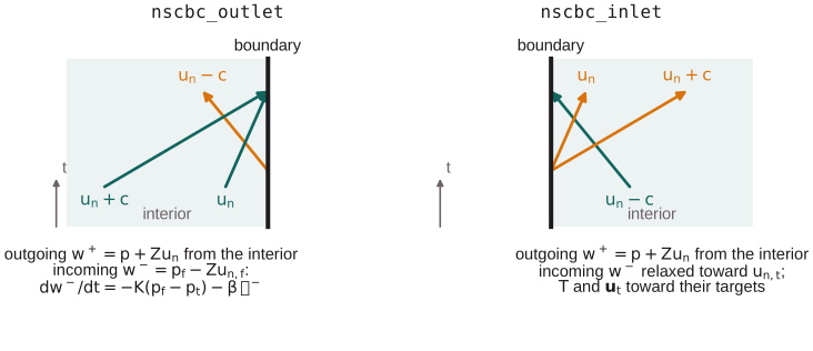
nscbc_outlet and nscbc_inlet are the non-reflecting boundaries of Poinsot & Lele 1992 in a weak, finite-volume form (src/numerics/characteristic.h; design notes). Each face keeps its own pressure and normal velocity \((p_f, u_{n,f})\), which define the incoming acoustic wave \(w^- = p_f - Z u_{n,f}\), \(Z = \rho c\). Once per step, \(w^-\) is advanced by one forward-Euler step of the LODI relation with relaxation toward a target and the transverse terms of Lodato, Domingo & Vervisch 2008 (Yoo & Im 2007); the outgoing wave \(w^+ = p + Z u_n\) comes from the reconstructed interior state averaged over the face:

\[ \begin{equation} \frac{\mathrm{d}w^-}{\mathrm{d}t} = \begin{cases} -K\,(p_f - p_t) - \beta\,\mathcal{T}^- & \text{outlets}, \\ K\,Z\,(u_{n,f} - u_{n,t}) - Z\,\dfrac{\mathrm{d}u_{n,t}}{\mathrm{d}t} - \beta\,\mathcal{T}^- & \text{inlets}, \end{cases} \qquad K = \min\left(\frac{\sigma}{L}\,c\,(1 - M^2),\ \frac{1}{\Delta t}\right), \label{eq:characteristic-boundaries-1} \end{equation} \]

with \(p_t\), \(u_{n,t}\) the targets, \(L\) = L the domain length, \(\sigma\) = sigma (default 0.25), \(M = \lvert\mathbf{u}\rvert/c\), and then \(p_f = \tfrac12(w^+ + w^-)\), \(u_{n,f} = (w^+ - w^-)/(2Z)\). A target that varies in time (synthetic turbulence) carries its own incoming wave, \(-Z\,\Delta u_{n,t}\) over the step, which enters without reflecting outgoing waves (Guézennec & Poinsot 2009). The transverse terms are

\[ \begin{equation} \mathcal{T}^- = \mathbf{u}_t\cdot\nabla_t p + c^2\rho\,\nabla_t\cdot\mathbf{u}_t - c\,\rho\,\mathbf{u}_t\cdot\nabla_t u_n, \label{eq:characteristic-boundaries-2} \end{equation} \]

with tangential derivatives from a least-squares fit, in the plane of the face, of the boundary cells of the neighboring characteristic faces (cell gradients would pick up the normal variation of waves crossing the boundary). \(\beta\) = beta defaults to the local Mach number (capped at 1), to 0 at turbulent inlets (whose target already carries its transverse terms) and on outlet faces with backflow; faces at the edge of the boundary (sharing a node with a wall) get none.

The exterior state for the Riemann solver (characteristic_W) combines the outgoing wave of the interior face state with the face's incoming wave:

\[ \begin{equation} p^b = \max\left(\tfrac12(w^+ + w^-),\ 10^{-3}p^L\right), \qquad u_n^b = \frac{w^+ - w^-}{2Z}, \label{eq:characteristic-boundaries-3} \end{equation} \]

with the remaining variables from the upwind side: for outflow (\(u_n \ge 0\)) the interior entropy, \(\rho^b = \rho^L(p^b/p^L)^{1/\gamma}\), and tangential velocity; for backflow at outlets the transmissive state's; for inflow at inlets the target, with temperature and tangential velocity relaxed from the transmissive state \(\mathbf{W}^e\) toward it,

\[ \begin{equation} T^b = T^e + a_T\,(T_t - T^e), \qquad \mathbf{u}_t^b = \mathbf{u}_t^e + a_t\,(\mathbf{u}_{t,t} - \mathbf{u}_t^e), \qquad a_{T,t} = \min\left(1,\ \frac{\sigma_{T,t}}{L}\,\frac{2d\,c}{-u_n}\right), \label{eq:characteristic-boundaries-4} \end{equation} \]

with \(2d\) twice the distance from the boundary cell's centroid to the face, \(\sigma_T\) = sigma_T and \(\sigma_t\) = sigma_t (imposed exactly, \(a = 1\), by default), and \(\rho^b = p^b/(R_t T^b)\) at the target's gas constant. Supersonic outflow takes \(\mathbf{W}^L\), supersonic inflow the target. The low-Mach correction applies at characteristic faces, and MUSCL boundary cells there reconstruct without the zero-gradient ghosts (chapter 5). An inlet's target velocity is per face and may carry synthetic turbulence (chapter 4).

Waves at characteristic boundaries

Sources¶

The sources are integrated over each cell before the division by its volume (src/solver/solver_rhs.cpp), except the sponges, which act on the rates afterwards.

Gravity¶

[source] gravity adds \(\mathbf{s}_u = \rho\,\mathbf{g}\), \(s_E = \rho\,\mathbf{u}\cdot\mathbf{g}\).

Expression sources¶

[source] rho, rhou and rhoE are per-volume sources given as expressions of \(\mathbf{x}\) and \(t\), evaluated at the cell centroids once, or at every stage with time_dependent = true.

Constant mass flow¶

With [source] mass_flow \(= \dot m\,\mathbf{e}\), a uniform body force along the unit vector \(\mathbf{e}\) holds the volume average of \(\rho\mathbf{u}\cdot\mathbf{e}\) at \(\dot m\). At every stage,

\[ \begin{equation} f = -\frac{1}{V}\sum_i \mathbf{R}_{\rho\mathbf{u},i}\cdot\mathbf{e} + \frac{1}{\Delta t}\left(\dot m - \frac{1}{V}\sum_i\lvert\Omega_i\rvert\,(\rho\mathbf{u})_i\cdot\mathbf{e}\right), \qquad \mathbf{s}_u = f\,\mathbf{e}, \qquad s_E = f\,\mathbf{e}\cdot\mathbf{u}, \label{eq:constant-mass-flow} \end{equation} \]

with \(V\) the domain volume and \(\mathbf{R}_{\rho\mathbf{u},i}\) the cell's integrated momentum rate from all other terms: the first part cancels their effect on the average, the second closes any remaining gap within the step.

Sponge layers¶

Sponge layers ([[sponges]]) relax the solution toward a target state \(\mathbf{U}_t\) (from u, p, T and, for mixtures, the composition, all possibly expressions) with a strength \(\sigma(\mathbf{x}) \ge 0\) (strength, 1/s):

\[ \begin{equation} \frac{\mathrm{d}\overline{\mathbf{U}}_i}{\mathrm{d}t} \mathrel{+}= \sigma_i\left(\mathbf{U}_{t,i} - \overline{\mathbf{U}}_i\right), \label{eq:sponge-layers} \end{equation} \]

for every conservative variable including the partial densities. Overlapping sponges add their strengths and average their targets weighted by strength. The time step is limited to \(\Delta t \le 1/\max_i\sigma_i\).

Radiation¶

[radiation] adds the optically thin loss of chapter 3, at every stage.

Axisymmetric source¶

Axisymmetric runs add the radial momentum source of chapter 1, integrated as in chapter 5.