Documentation of the main branch
These pages follow Mallard's main branch, which is ahead of release 0.8.0: some features they describe come with the next release.
Chemistry and radiation¶
This chapter gives the chemical source terms \(\dot\omega_k\) of eq. (2) of chapter 1, the
stiff integrator that advances them, how they are coupled to the flow by
operator splitting, and the optically thin radiation model. Chemistry needs
a gas mixture (chapter 2) and a [chemistry]
table. Usage: Thermochemistry; measured
splitting errors: Numerical methods.
Finite-rate kinetics¶
Mallard reads the reactions of a Cantera YAML phase and evaluates them as
Cantera does (Kee, Coltrin & Glarborg 2003;
src/chemistry/kinetics.h), in SI units with kmol, in double precision.
With concentrations \(C_k = \rho Y_k/W_k\), reaction \(j\) with reactant and
product stoichiometric coefficients \(\nu'_{kj}\), \(\nu''_{kj}\) has the rate of
progress
with forward orders \(o_{kj} = \nu'_{kj}\) unless the mechanism gives other (possibly non-integer) orders. The production rates and the heat release rate are
Rate constants¶
The basic form is the modified Arrhenius law,
Depending on the reaction type, \(k_{f,j}\) is
- elementary: eq. \(\eqref{eq:rate-constants-1}\);
- three-body: eq. \(\eqref{eq:rate-constants-1}\) times \([M] = \sum_k \epsilon_{kj} C_k\), with efficiency 1 unless the mechanism gives another (this multiplies both directions);
-
falloff: with \(k_0\) and \(k_\infty\) the low- and high-pressure limits (each eq. \(\eqref{eq:rate-constants-1}\)) and the reduced pressure \(P_r = k_0[M]/k_\infty\),
\[ \begin{equation} k_f = k_\infty\,\frac{P_r}{1 + P_r}\,F(T, P_r), \label{eq:rate-constants-2} \end{equation} \]where \(F = 1\) (Lindemann), or Troe's form (Gilbert, Luther & Troe 1983),
\[ \begin{equation} \begin{aligned} F_\mathrm{cent} &= (1 - \alpha)\,e^{-T/T_3} + \alpha\,e^{-T/T_1} + e^{-T_2/T}, \\ \log_{10} F &= \frac{\log_{10} F_\mathrm{cent}}{1 + \left(\dfrac{\log_{10}P_r + c}{n - 0.14\,(\log_{10}P_r + c)}\right)^2}, \qquad c = -0.4 - 0.67\log_{10}F_\mathrm{cent}, \quad n = 0.75 - 1.27\log_{10}F_\mathrm{cent}, \end{aligned} \label{eq:rate-constants-3} \end{equation} \]where a term is dropped when its \(T_3\), \(T_1\) or \(T_2\) is absent, or the SRI form (Stewart, Larson & Golden 1989),
\[ \begin{equation} F = d\left(a\,e^{-b/T} + e^{-T/c}\right)^{X} T^{e}, \qquad X = \frac{1}{1 + (\log_{10}P_r)^2}; \label{eq:rate-constants-4} \end{equation} \] -
PLOG: \(\ln k\) interpolated linearly in \(\ln p\) between the two bracketing pressures of the table (the rates given at one pressure are summed), and held constant beyond its ends;
- Chebyshev: \(\log_{10}k = \sum_{t}\sum_{q}\alpha_{tq}\,\phi_t(\tilde T)\,\phi_q(\tilde p)\) with Chebyshev polynomials \(\phi\) of the reduced variables \(\tilde T = (2T^{-1} - T_\mathrm{min}^{-1} - T_\mathrm{max}^{-1})/(T_\mathrm{max}^{-1} - T_\mathrm{min}^{-1})\) and \(\tilde p = (2\ln p - \ln p_\mathrm{min} - \ln p_\mathrm{max})/(\ln p_\mathrm{max} - \ln p_\mathrm{min})\).
PLOG and Chebyshev reactions use the pressure \(p = R_u T\sum_k C_k\).
Reverse rates¶
Reversible reactions take \(k_{r,j} = k_{f,j}/K_{c,j}\), with the equilibrium constant from the molar standard Gibbs energies \(\hat g_k^\circ = W_k(h_k - T s_k^\circ)\) of eq. (1) of chapter 2,
with \(p_\mathrm{atm}\) = 101325 Pa, the standard state of the data. Irreversible reactions have \(k_r = 0\).
Fractional orders¶
A non-integer order \(0 < o < 1\) makes \(C^o\) infinitely steep at \(C = 0\),
which stiff integrators cannot follow. Below \(C_\mathrm{reg}\)
([chemistry] C_reg, default \(10^{-12}\) kmol/m³) the factor is replaced
by a quadratic in \(x = C/C_\mathrm{reg}\) that joins \(C^o\) with a continuous
slope at \(C_\mathrm{reg}\) and has a bounded slope at zero:
Other non-integer orders use \(\max(C, 0)^o\).
Reactor equations¶
Each cell's chemistry is an adiabatic, constant-volume reactor at its
density: over a chemistry substep \(\rho\), \(\rho\mathbf{u}\) and \(\rho E\) are
fixed, and since \(e\) includes the enthalpies of formation
(chapter 2) the
specific internal energy is constant. The state
\(\mathbf{y} = (Y_1,\dots,Y_{N_s}, T)\) obeys (ConstantVolumeReactor,
src/chemistry/reactor.h)
with \(e_k = h_k - R_u T/W_k\) the species internal energies. The Jacobian
\(\partial\mathbf{f}/\partial\mathbf{y}\) is analytical: the derivatives of
every rate of progress with respect to \(T\) and to each concentration
(including those through \([M]\), \(P_r\) and the pressure of PLOG and
Chebyshev reactions) are assembled by the chain rule. Mechanisms of 30
species or more whose factored Jacobian pattern fills at most 60% of the
dense matrix use a sparse LU, with the dependence on the total
concentration as a rank-one update; others a dense LU with partial
pivoting ([chemistry] sparse overrides the choice).
Before integrating, negative mass fractions are clipped to zero and the composition renormalized, with \(T\) recomputed at the same \(e\); after it, the mass fractions are clipped and renormalized again and \(T\) follows from the initial \(e\), so energy is conserved exactly. Only the partial densities of the cell change.
Cells are skipped where nothing would happen: a cell reacts only if
\(T \ge T_\mathrm{frozen}\) (T_frozen, default 0) and
at its current state, with \(\mathrm{atol}\) the absolute tolerance of the mass fractions below.
Stiff integration: RODAS¶
Eq. \(\eqref{eq:reactor-equations-1}\) is integrated by RODAS
(Hairer & Wanner 1996, §IV.7), a
stiffly accurate, L-stable Rosenbrock method of order 4 with an embedded
order-3 solution, with \(\gamma = 1/4\) and the coefficients of rodas.f
(src/chemistry/rosenbrock.h). A step of size \(h\) from \(\mathbf{y}_0\)
solves six linear systems with the one matrix
\(\mathbf{A} = \mathbf{I}/(\gamma h) - \mathbf{J}\),
\(\mathbf{J} = \partial\mathbf{f}/\partial\mathbf{y}(\mathbf{y}_0)\):
except that stage 6 is evaluated at \(\mathbf{y}_0 + \sum_{l\le 4} a_{5l}\mathbf{k}_l + \mathbf{k}_5\). The solution is \(\mathbf{y}_1 = \mathbf{y}_0 + \sum_{l\le 4} a_{5l}\mathbf{k}_l + \mathbf{k}_5 + \mathbf{k}_6\) (stiffly accurate) and \(\mathbf{k}_6\) is the error estimate. A step is accepted when the new state is admissible (no mass fraction below \(-\mathrm{atol}\), positive \(T\)) and
with \(\mathrm{rtol}\) = rtol (default \(10^{-6}\)),
\(\mathrm{atol}_i\) = atol (default \(10^{-10}\)) for the mass fractions and
0 for \(T\). The next step is
capped at \(h\) right after a rejection. A rejected step retries with
\(h\max(0.2, 0.9\,\mathrm{err}^{-1/4})\), or with \(h/4\) if \(\mathbf{A}\) is
singular or the state inadmissible. Each cell keeps its last proposed \(h\)
for its next call (first guess \(10^{-7}\) s); a call fails after max_steps
(default \(10^5\)) accepted and rejected sub-steps, or when \(h\) falls below
\(10^{-14}\) of the interval.
Coupling with the flow¶
Strang splitting¶
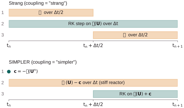
By default ([chemistry] coupling = "strang"), each time step is the
symmetric sequence (Strang 1968;
Solver::take_step, src/solver/solver.cpp)
where \(\mathcal{R}_\tau\) integrates eq. \(\eqref{eq:reactor-equations-1}\) in every cell over \(\tau\) and
\(\mathcal{T}_{\Delta t}\) is one step of the explicit time integrator on the
flow's right-hand side (fluxes, sources, sponges, radiation;
chapter 7). With fuse_half_steps = true the
trailing half step of one time step and the leading half step of the next
are fused into one call over \(\Delta t\), except where output, checks or the
end of the run read the state at a step boundary. The splitting is second
order, but its fixed point moves with \(\Delta t\).
SIMPLER balanced splitting¶
With coupling = "simpler", Mallard uses the SIMPLER scheme of
Wu, Ma & Ihme 2019 (their eqs. 3.18;
Solver::take_simpler_step). With \(\mathcal{T}(\mathbf{U})\) the flow's
right-hand side and \(\mathcal{R}(\mathbf{U})\) the chemical one,
The reaction substep runs over the whole step with the transport tendency as a constant source; the transport substep is one step of the explicit integrator over the second half of the step on \(\mathcal{T}(\mathbf{U}) - \mathcal{T}(\mathbf{U}^n)\). The half length makes the scheme second order. A steady state of the full system, \(\mathcal{R}(\mathbf{U}^n) + \mathcal{T}(\mathbf{U}^n) = 0\), is a fixed point at every \(\Delta t\).
In the reaction substep every cell's \(\rho\), \(\rho\mathbf{u}\) and \(\rho E\) move to \(\mathbf{U}^n + \Delta t\,\mathcal{T}(\mathbf{U}^n)\). A cell whose chemistry is active (eq. \(\eqref{eq:reactor-equations-2}\)) at \(\mathbf{U}^n\) or at that end state integrates the forced reactor: with \(y_k = \rho Y_k/\rho^n\), \(g_k = \mathcal{T}_{\rho Y_k}(\mathbf{U}^n)/\rho^n\) and \(g_e\) the constant rate of change of the internal energy per unit initial mass between \(\mathbf{U}^n\) and the end state,
an autonomous system whose species rows of the Jacobian are those of
eq. \(\eqref{eq:reactor-equations-1}\). Sub-steps are rejected only below
\(y_k = -\mathrm{atol} - \Delta t\max(0, -g_k)\), since a forcing that
removes a species can drive the exact solution that far below zero. The end
mass fractions are clipped and renormalized at the end density; other cells
take the forward-Euler update of their partial densities. Without chemistry
a SIMPLER step is therefore \(\mathbf{U}^n + \Delta t\,\mathcal{T}(\mathbf{U}^n)\)
followed by the integrator over \(\Delta t/2\), which changes the
integrator's stability polynomial (with SSPRK3, \(1 + z + z^2/2 + z^3/8 + z^4/48\)):
stable with upwind fluxes but not on the imaginary axis, so SIMPLER rejects
the non-dissipative hybrid flux, as well as double_flux and
fuse_half_steps (design notes).
With TFLES or PaSR (chapter 4), a cell's reaction rates are scaled by a factor \(s\): its reactor is integrated over \(s\,\tau\) instead (with forcing \(\mathbf{g}/s\)), which is the same ODE.
Optically thin radiation¶
[radiation] (gas mixtures) adds the optically thin radiative loss of the
TNF workshop model (Barlow et al. 2001;
Grosshandler 1993;
src/chemistry/radiation.h) to the energy equation, as a sink in the
flow's right-hand side evaluated at every stage:
with \(\sigma_{SB}\) the Stefan-Boltzmann constant, \(T_\mathrm{amb}\) =
T_ambient (default 300 K), \(p_i\) the partial pressures in atm and
\(a_{P,i}\) the Planck-mean absorption coefficients (1/(m atm)) of the
radiating species present in the mechanism (H2O, CO2, CO and CH4, or those
listed in species), fitted to RADCAL over 300-2500 K:
with \(T\) in kelvin. The gas neither absorbs radiation from elsewhere nor scatters it: the model suits small, optically thin flames.