Documentation of the main branch

These pages follow Mallard's main branch, which is ahead of release 0.8.0: some features they describe come with the next release.

Turbulent channel flow (LES)¶

Turbulent flow between two parallel walls, driven by a constant mass flow, is the canonical wall-bounded flow: its statistics depend only on the friction Reynolds number Re_τ = u_τ h / ν, and the direct numerical simulations of Moser, Kim & Mansour (1999) give them at Re_τ = 180, 395 and 590. This tutorial runs a wall-resolved large-eddy simulation at Re_τ = 180 on a mesh of 49,000 hexahedra from Gmsh, follows the flow from laminar-like rolls to turbulence, collects time averages, and compares the mean velocity and Reynolds stresses with the DNS.

You will use: a structured hexahedral Gmsh mesh with periodic zones ([[periodic]]), an initial state as expressions of x, y and z, the constant-mass-flow forcing, the Sigma subgrid model and the kinetic-energy-preserving hybrid flux, running statistics ([statistics]), the dissipation budget of [integrals], and restart files. Files: tutorials/channel_les/. Setup: Tutorials.

1. Geometry¶

Walls at y = 0 and y = 2h; the flow is periodic in x and z over a box of 2πh × 2h × πh, long and wide enough for the largest near-wall structures at this Reynolds number. In units of h and of the bulk density and velocity U_b, the bulk Reynolds number 2 h U_b / ν = 5600 of the DNS fixes μ = 3.57e-4; the friction velocity, and so Re_τ, comes out of the run.

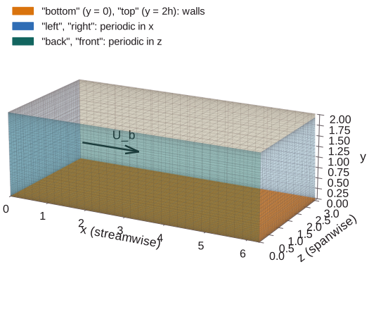
The channel box and its boundary zones: walls at bottom and top, periodic pairs in x and z

2. Mesh¶

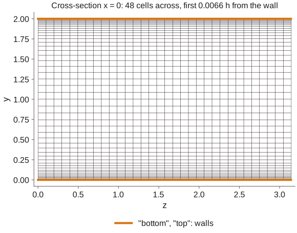
channel.geo extrudes a line of nodes along y, clustered toward both walls with Mallard's tanh law (the same nodes as [mesh] stretching gives a generated box), first along x, then along z. Extrusion makes the faces at x = 0 and x = 2πh carry the same nodes translated, as [[periodic]] needs.

mkdir -p run/channel_les && cd run/channel_les
cp $MALLARD/tutorials/channel_les/input.toml .
gmsh $MALLARD/tutorials/channel_les/channel.geo -3 -o channel.msh    # 32 x 48 x 32
python3 $MALLARD/tutorials/channel_les/plot_channel_les.py mesh channel.msh --out .

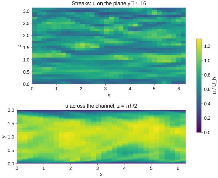
With Re_τ ≈ 180 the cells are Δx⁺ = 35 and Δz⁺ = 18 apart, Δy⁺ = 1.2 at the wall and 16 at the center: a coarse wall-resolved LES, which resolves the near-wall streaks but not their finest scales and leaves those to the subgrid model.

Cross-section of the mesh: 48 cells across the channel, clustered at the walls

3. Input file¶

Table	In this case
`[run]`	`t_stop = 300` h/U_b, at CFL 0.9
`[mesh]`, `[[periodic]]`	`channel.msh`; `left`/`right` joined with `translation = [2π, 0, 0]`, `back`/`front` with `[0, 0, π]`: their faces become interior and need no `[[boundaries]]`
`[initialize]`	`analytical`: the turbulent-like mean profile (8/7)(1 − \|y − 1\|)^(1/7), whose bulk velocity is 1, plus streamwise and spanwise rolls of about 15% of U_b, divergence-free and zero at the walls, written as expressions of x, y and z
`[[boundaries]]`	`bottom`, `top`: `wall_isothermal` at the bulk temperature, which carries away the heat of dissipation
`[source]`	`mass_flow = [1, 0, 0]`: a uniform body force holds the bulk mass flow at 1
`[numerics]`	`convective_flux = "hybrid"`: the kinetic-energy-preserving central flux, with HLLC only at compressions (there are none here); unlimited MUSCL states
`[physics]`	`navier_stokes`, bulk Mach number 0.2 (`p_ref = 1/(γ M²)`)
`[les]`	`model = "sigma"` with Scotti's filter width for the stretched cells
`[statistics]`	Running means of ρ, u, p, T and the covariances u'u', v'v', w'w', u'v', every 10 steps from t = 100
`[integrals]`	`budget = true`: the dissipation of kinetic energy split into molecular, subgrid and numerical parts
`[[forces]]`	The force on each wall: its viscous x-component is the wall shear
`[[write_data]]`	Every 50 h/U_b: the flow (u, p, the Q-criterion, the eddy viscosity), the statistics, and a restart file

4. Run¶

The time step is set by the acoustic speed in the thin wall cells (1e-3 h/U_b), so 300 h/U_b is 300,000 steps: under an hour on one A100, and hours on a CPU.

$MALLARD/build-3d/src/Mallard -i input.toml --kokkos-num-threads=8    # CPU threads
mpirun -n 4 $MALLARD/build-3d/src/Mallard -i input.toml               # MPI ranks

A run that stops (a time limit, t_wall_stop, or a crash) continues from its last restart file, statistics included, bit for bit: set [initialize] to type = "restart" and file = "restart/channel_<step>.restart".

5. Monitor¶

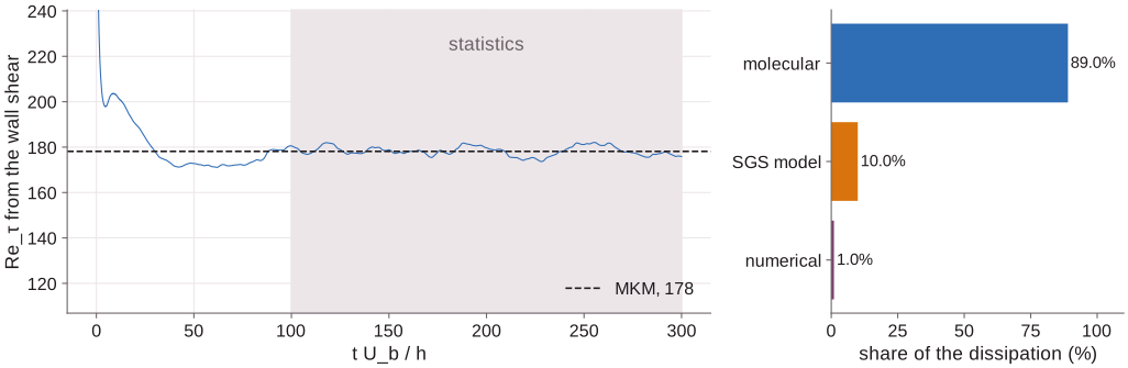
The rolls break down into turbulence within the first 30 h/U_b, and Re_τ settles by t ≈ 90. The wall shear, which sets Re_τ, is in forces_bottom.csv and forces_top.csv as the run goes; integrals.csv has the kinetic energy and the dissipation budget. The statistics should start only once Re_τ has settled (t = 100 here) and run long enough to converge the averages: here 200 h/U_b, about 13 h/u_τ.

Re_tau from the wall shear over time, and the shares of the dissipation

Streamwise velocity on a plane near the wall, showing the streaks, and across the channel

6. Post-process and compare¶

python3 $MALLARD/tutorials/channel_les/plot_channel_les.py results . --t-start 100 --out .

averages the last statistics snapshot over x and z (with tools/plane_average.py, which also adds the dispersive part of the covariances), folds the two halves of the channel, takes u_τ from the wall shear averaged over the same window, and compares in wall units with the DNS, downloaded on first use:

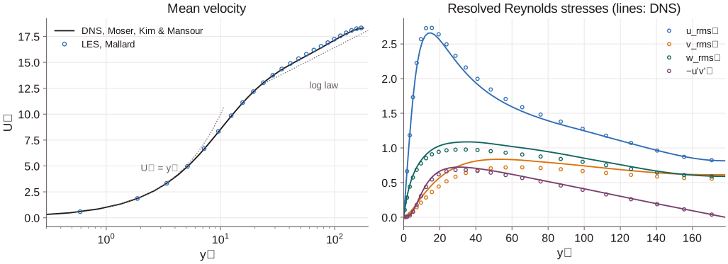
averaging window t = 100 to 299.954 h/U_b (12.7 h/u_tau)
Re_tau = 178.3 (MKM 178.1, +0.1%), Cf = 0.00807 (MKM 0.00814, -0.8%)
peak u_rms+ 2.732 at y+ = 15.6 (MKM 2.658 at 15.3)
peak v_rms+ 0.720 at y+ = 65.7 (MKM 0.836 at 52.2)
peak w_rms+ 0.976 at y+ = 34.4 (MKM 1.087 at 35.1)
peak -u'v'+ 0.682 at y+ = 34.4 (MKM 0.723 at 30.0)
U+(10) = 8.56 (MKM 8.52)
U+(30) = 13.89 (MKM 13.87)
U+(100) = 17.26 (MKM 17.15)
dissipation: molecular 89.0%, SGS 10.0%, numerical 1.0%

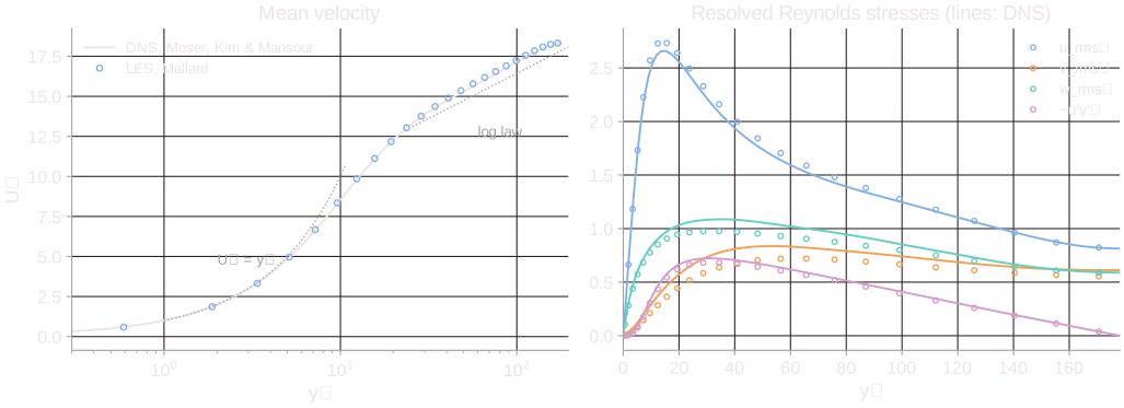
Re_τ and the skin friction are within 1% of the DNS and the mean velocity within 1% across the channel. The fluctuations are the resolved part only: u_rms is 3% high at its peak, and v_rms and w_rms are 10-14% low, the energy of the scales the mesh does not resolve (finer meshes in x and z recover it). The subgrid model takes 10% of the dissipation and the central scheme 1%, so the model, not the numerics, does the work of the unresolved scales.

Mean velocity and resolved Reynolds stresses in wall units against the DNS

7. Higher Reynolds numbers and wall models¶

The cost of a wall-resolved LES grows steeply with the Reynolds number, since the near-wall cells must shrink with the viscous length ν / u_τ: examples/channel_les runs Re_τ = 395 and 590 on 64³ and 96³ cells. Wall-modeled LES removes that constraint by modeling the inner layer and resolving only the outer flow; it is under development for Mallard (issue #256). This tutorial is set up for it: its mesh is the channel.geo of this page with a uniform or mildly stretched spacing in y (-setnumber beta 0.5), and its input this one at a higher bulk Reynolds number, with the wall model's table in place of the wall-resolution requirement. This section will walk through it once the wall model is merged.

8. Things to try¶

No model. Remove [les]: with the central flux the only dissipation left at the grid scale is numerical, and Re_τ comes out several percent high (see examples/channel_les).
Resolution. -setnumber nx 64 -setnumber nz 64 halves Δx⁺ and Δz⁺.
Riemann solver everywhere. convective_flux = "riemann" and compare the numerical share of the dissipation.