Documentation of the main branch

These pages follow Mallard's main branch, which is ahead of release 0.8.0: some features they describe come with the next release.

Physics¶

[physics] chooses the equations (Euler or Navier–Stokes), the gas (a single calorically perfect gas, or a thermally perfect mixture of species) and the geometry (planar or axisymmetric).

Euler and Navier–Stokes¶

[physics]
type = "navier_stokes"   # or "euler" (the default)
gamma = 1.4
p_ref = 1.0              # any state of the gas: sets R = p_ref / (rho_ref T_ref)
T_ref = 1.0
rho_ref = 1.0
mu = 1.0e-3              # navier_stokes: dynamic viscosity
Pr = 0.72

Key	Default	Meaning
`type`	`"euler"`	`euler` (inviscid) or `navier_stokes` (viscous, heat-conducting)
`gamma`	required	Ratio of specific heats
`p_ref`, `T_ref`, `rho_ref`	required	A reference state; only the gas constant `R = p_ref / (rho_ref T_ref)` is taken from it
`mu`	required (`navier_stokes`)	Dynamic viscosity, or its value at `T_mu_ref` for the temperature-dependent laws
`Pr`	0.72	Prandtl number; the conductivity is `cp mu / Pr`
`viscosity_model`	`"constant"`	`constant`, `sutherland` or `power_law`
`T_mu_ref`	273.15 (`sutherland`); required (`power_law`)	Temperature at which the viscosity is `mu`
`sutherland_S`	110.4	Sutherland temperature
`viscosity_exponent`	required (`power_law`)	`mu (T / T_mu_ref)^viscosity_exponent`
`gas`	`"perfect"`	`perfect` or `mixture` (Thermochemistry)
`axisymmetric`	`false`	2D only: flows symmetric about the x axis, below

When to use which:

Euler for shock-dominated flows where viscosity does not matter at the scales of the mesh (shock tubes, blast waves, detonation fronts); the wall_* conditions are then slip walls.
Navier–Stokes for boundary layers, wakes and turbulence: walls are no-slip, the time step includes the viscous limit, and the large-eddy simulation models add to the molecular viscosity.

Mallard is scale-free for a single gas: the reference state only fixes R, so the common nondimensionalization (free-stream density and sound speed 1, or p_ref = T_ref = rho_ref = 1) works as it is. The cylinder example, for instance, takes the cylinder diameter and free-stream sound speed as units, so U = M = 0.2 and mu = U D / Re.

Viscosity laws¶

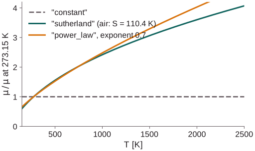
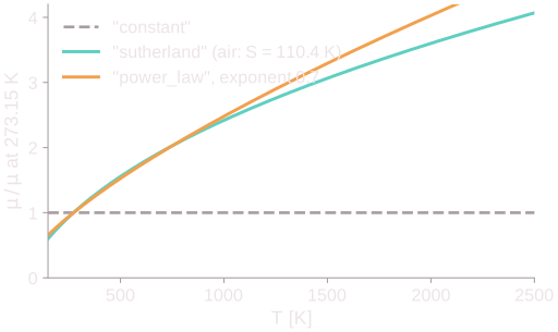
Viscosity against temperature for the constant, Sutherland and power laws

viscosity_model = "sutherland"   # air: mu(T) = mu (T / T_mu_ref)^1.5 (T_mu_ref + S) / (T + S)
mu = 1.716e-5                    # at T_mu_ref = 273.15 K

Use Sutherland's law (or a power law) when the temperature varies by more than tens of percent: shock-heated boundary layers, the viscous shock tube, hot wakes. A constant viscosity is right for nearly isothermal flows and for comparisons with incompressible references.

Gas mixtures¶

gas = "mixture" replaces gamma and the reference state with the species of a Cantera mechanism: thermally perfect thermodynamics, mixture-averaged or simpler transport, and finite-rate chemistry with [chemistry]. See Thermochemistry.

Axisymmetric flows¶

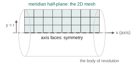
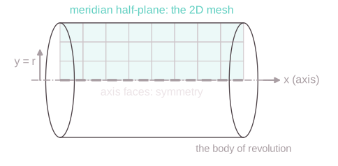
With axisymmetric = true (2D builds), the mesh is the meridian half-plane of a body of revolution: x is the axis and y the radius, so every node needs y >= 0. Each cell stands for the solid it sweeps around the axis; there is no swirl.

The 2D mesh as the meridian half-plane of a body of revolution about the x axis

[physics]
type = "navier_stokes"
axisymmetric = true
# ...

[[boundaries]]
name = "axis"            # every boundary face on y = 0
type = "symmetry"

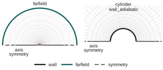
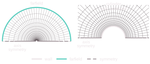
The meridian half-plane of the axisymmetric sphere example with its zones

examples/sphere_axisymmetric: flow past a sphere at Re = 100 and 150 on a half O-grid (make_cylinder_mesh.py --half, drawn coarser than it runs).

Boundary faces on the axis must be symmetry; nothing crosses them.
u is [u_x, u_r]. Cell values are r-weighted averages, and analytical initial conditions are averaged that way.
Fluxes, sources, forces ([[forces]]), [integrals] and conserved totals are per radian: multiply a force by 2 pi for the force on the body; only its axial component is meaningful.
Every reconstruction, Riemann solver, viscous and mixture model, chemistry and MPI work as in planar runs, at design order up to the axis.
Not available: periodicity in y, curved boundaries, and [les] (planar runs only).

Examples, each checked against an exact or reference solution: poiseuille_pipe, noh_axisymmetric, sedov_axisymmetric and sphere_axisymmetric.