Documentation of the main branch

These pages follow Mallard's main branch, which is ahead of release 0.8.0: some features they describe come with the next release.

Finite-volume discretization and reconstruction

Mallard discretizes eq. (3) of chapter 1 with a cell-centered finite-volume method on unstructured meshes: triangles and quadrilaterals in 2D, tetrahedra, hexahedra, prisms and pyramids in 3D, with optionally curved boundary faces. This chapter covers the semi-discrete equations, face quadrature, curved geometry, the reconstruction of face states (first order, MUSCL, TENO-E), the low-Mach correction of those states and the cell gradients of the viscous terms. The numerical fluxes are in chapter 6 and the time integration in chapter 7. Usage: Numerics; measured stability and accuracy limits: Numerical methods.

Semi-discrete equations

The unknowns are the cell averages \(\overline{\mathbf{U}}_i = \lvert\Omega_i\rvert^{-1}\int_{\Omega_i}\mathbf{U}\,\mathrm{d}V\). Integrating eq. (3) of chapter 1 over cell \(i\),

\[ \begin{equation} \frac{\mathrm{d}\overline{\mathbf{U}}_i}{\mathrm{d}t} = -\frac{1}{\lvert\Omega_i\rvert}\sum_{f\in\partial\Omega_i} s_{i,f}\left(\mathbf{F}_f - \mathbf{F}^v_f\right) + \overline{\mathbf{S}}_i, \label{eq:semi-discrete-equations-1} \end{equation} \]

where \(s_{i,f} = +1\) if \(i\) is the face's first cell (the normal \(\mathbf{n}_f\) points out of \(i\)) and \(-1\) otherwise, and \(\mathbf{F}_f\), \(\mathbf{F}^v_f\) are the convective and viscous fluxes integrated over the face:

\[ \begin{equation} \mathbf{F}_f = \frac{A_f}{2}\sum_{q} w_{f,q}\,\hat{\mathbf{F}}\left(\mathbf{U}^L_{f,q}, \mathbf{U}^R_{f,q}; \mathbf{n}_{f,q}\right), \label{eq:semi-discrete-equations-2} \end{equation} \]

with face weights normalized to \(\sum_q w_{f,q} = 2\) (Gauss-Legendre on \([-1, 1]\) in 2D; 3D rules rescaled to that sum). The viscous flux uses one point per face (chapter 6). Each face's flux is computed and stored once, and every cell sums its faces in a fixed order without atomic operations (FaceFluxSumFunctor, src/numerics/flux_functor.h), so the result is bitwise independent of thread count and scheduling. Boundary faces use the exterior state of the boundary condition as \(\mathbf{U}^R\) (chapter 8). The source term is evaluated at the cell average.

Face quadrature

On straight faces the quadrature points and weights are (src/numerics/quadrature.cpp, face_reconstruction.cpp):

Reconstruction	2D edges	3D triangles	3D quadrilaterals
First order, MUSCL	1 point (midpoint)	centroid	centroid
TENO-E, order 3 or 4	Gauss-Legendre, 2 points	Dunavant rule of degree 4	tensor Gauss-Legendre, 2 × 2 points, bilinear map
TENO-E, order 5 or 6	Gauss-Legendre, 3 points	Dunavant rule of degree 5	tensor Gauss-Legendre, 3 × 3 points, bilinear map

so that the reconstructed polynomial, of degree one less than the order, is integrated exactly over straight faces (Dunavant 1985). Each face has one unit normal \(\mathbf{n}_f\), except curved faces, which have one per point.

Curved boundaries

A straight cell next to a curved wall misplaces it by \(O(h^2/R)\), which caps the order of the scheme. With high-order Gmsh boundary elements or an analytic shape on a boundary zone ([[mesh.curved]]: circle, sphere or cylinder), boundary faces follow the curved geometry (src/mesh/curved.cpp; design notes).

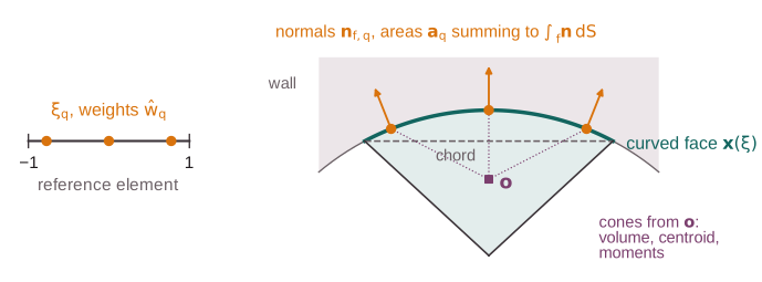
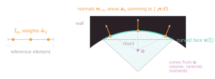
Face maps. A curved face is a map \(\mathbf{x}(\boldsymbol{\xi})\) from its flat reference element. Analytic shapes project a point of the straight face radially onto the shape, minus the linear interpolant of the corners' projection offsets, so that faces still meet at the mesh nodes. Gmsh elements of order 2 or 3 give Lagrange edges, plus interior nodes. In 3D, every face sharing an edge with a curved face is blended from its edges: on triangles \(\mathbf{x} = \mathbf{x}_\mathrm{lin} + \sum_e \lambda_i\lambda_j\,\mathbf{q}_e(t)\), \(t = (1 + \lambda_j - \lambda_i)/2\), with \(\lambda\) the barycentric coordinates and \(\mathbf{q}_e\) the edge's deviation from its chord; on quadrilaterals a Coons patch.

Face quadrature. The flat rule \((\boldsymbol{\xi}_q, \hat w_q)\) is mapped through the face map. Each point gets the area vector \(\mathbf{a}_q = \hat w_q\,(\partial_u\mathbf{x}\times\partial_v\mathbf{x})(\boldsymbol{\xi}_q)\) (in 2D, the rotated tangent), and all area vectors are shifted by one common vector so that they sum exactly to the face's area vector,

\[ \begin{equation} \sum_q \mathbf{a}_q = \int_f \mathbf{n}\,\mathrm{d}S = \frac12\oint_{\partial f}\mathbf{x}\times\mathrm{d}\mathbf{x}, \label{eq:curved-boundaries} \end{equation} \]

which is exact for the face's curved edges. Every cell then still closes, \(\sum_f s_{i,f}\int_f\mathbf{n}\,\mathrm{d}S = 0\), and gas at rest stays at rest to round-off. Each point carries the unit normal \(\mathbf{n}_{f,q} = \mathbf{a}_q/\lvert\mathbf{a}_q\rvert\) and the weight \(w_{f,q} = 2\lvert\mathbf{a}_q\rvert/A_f\) in eq. \(\eqref{eq:semi-discrete-equations-2}\), where \(A_f\) is the length of the face's area vector.

Cells. Cells with a curved face are integrated over signed cones from their vertex average \(\mathbf{o}\) to each face, \(\mathbf{x} = \mathbf{o} + \tau\left(\mathbf{x}_f(\boldsymbol{\xi}) - \mathbf{o}\right)\), \(\tau\in[0, 1]\), with tensor Gauss rules over the curved faces. These rules give the volume, the centroid, the TENO-E moments and the initial cell averages of curved cells, exactly for polynomials.

Reconstruction

The face states \(\mathbf{U}^L\), \(\mathbf{U}^R\) at each quadrature point come from polynomials reconstructed from the cell averages around each cell ([numerics.face_reconstruction] type). A single gas reconstructs the variables named below; a gas mixture reconstructs \(\mathbf{W} = [\rho, \mathbf{u}, p]\) and its scalars separately (below). Boundary faces reconstruct only the interior side.

First order

\(\mathbf{U}^L_{f,q} = \overline{\mathbf{U}}_i\): piecewise constant.

MUSCL

MUSCL (van Leer 1979; src/numerics/face_reconstruction.cpp) reconstructs the primitive variables \(\mathbf{W} = [\rho, \mathbf{u}, p]\) linearly, with one point per face at its centroid \(\mathbf{x}_f\):

\[ \begin{equation} \mathbf{W}^L_f = \mathbf{W}_i + \boldsymbol{\phi}_i\circ\left(\nabla\mathbf{W}_i\cdot(\mathbf{x}_f - \mathbf{x}_i)\right), \label{eq:muscl-1} \end{equation} \]

with one limiter value per variable and cell. A face side whose density or pressure would be non-positive takes the cell value instead.

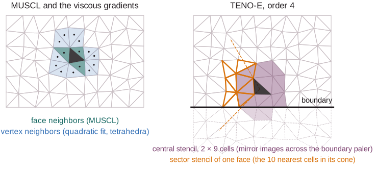
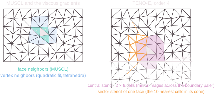
Gradients. Weighted least squares (Mavriplis 2003): with neighbor offsets \(\Delta\mathbf{x}_j = \mathbf{x}_j - \mathbf{x}_i\) and weights \(w_j = \lvert\Delta\mathbf{x}_j\rvert^{-2}\), \(\nabla W_i\) minimizes \(\sum_j w_j\left(W_j - W_i - \nabla W_i\cdot\Delta\mathbf{x}_j\right)^2\),

\[ \begin{equation} \left(\sum_j w_j\,\Delta\mathbf{x}_j\Delta\mathbf{x}_j^T\right)\nabla W_i = \sum_j w_j\,\Delta\mathbf{x}_j\,(W_j - W_i). \label{eq:muscl-2} \end{equation} \]

The neighbors are the face neighbors. A boundary face contributes its ghost state (chapter 8) at the mirror image of the cell centroid, \(\Delta\mathbf{x} = 2 d\,\mathbf{n}_f\) with \(d\) the centroid's distance to the face; prescribed states (dirichlet, upt, farfield) sit at the face centroid instead. Tetrahedra, whose four face neighbors make weakly limited MUSCL unstable, and cells on characteristic boundaries, whose zero-gradient ghosts would halve outgoing waves, use the linear fit over their vertex neighbors instead (the same fit as eq. \(\eqref{eq:muscl-2}\) over the vertex-neighbor stencil of below).

Limiters. With \(\Delta_{-} = \nabla W_i\cdot(\mathbf{x}_f - \mathbf{x}_i)\) at each face centroid and \(\Delta_{\max}\), \(\Delta_{\min}\) the largest and smallest \(W_j - W_i\) over the cell and its face neighbors (ghosts included), \(\phi_i = \min_f\phi_f\) with (Barth & Jespersen 1989; Venkatakrishnan 1995)

\[ \begin{equation} \phi_f^\mathrm{BJ} = \begin{cases} \min\left(1, \Delta_{\max}/\Delta_{-}\right) & \Delta_{-} > 0, \\ \min\left(1, \Delta_{\min}/\Delta_{-}\right) & \Delta_{-} < 0, \\ 1 & \Delta_{-} = 0, \end{cases} \qquad \phi_f^\mathrm{V} = \frac{\Delta_{+}^2 + \varepsilon^2 + 2\Delta_{-}\Delta_{+}}{\Delta_{+}^2 + 2\Delta_{-}^2 + \Delta_{-}\Delta_{+} + \varepsilon^2}, \label{eq:muscl-3} \end{equation} \]

where \(\Delta_{+} = \Delta_{\max}\) if \(\Delta_{-} > 0\) and \(\Delta_{\min}\) otherwise, and the Venkatakrishnan threshold (the default limiter) is

\[ \begin{equation} \varepsilon^2 = (K h_i)^3\,s^2, \qquad h_i = \lvert\Omega_i\rvert^{1/d}, \label{eq:muscl-4} \end{equation} \]

with \(K\) = venkatakrishnan_K (default 5) and the scale \(s\) of the variable: \(\rho_i\) for density, \(p_i\) for pressure, the sound speed \(a_i\) for the velocity components.

TENO-E

type = "TENO" with order \(k = 3,\dots,6\) is the TENO-E scheme of Liang, Shyy & Fu 2025, built on TENO (Fu, Hu & Adams 2016) and its unstructured finite-volume form (Ji, Liang & Fu 2022), extended to 3D cells (src/numerics/teno.cpp, teno_setup.cpp). Implementation details and measured stability cases: TENO-E details.

Polynomials. In the cell-scaled frame \(\boldsymbol{\xi} = (\mathbf{x} - \mathbf{x}_i)/h_i\), \(h_i = \lvert\Omega_i\rvert^{1/d}\), a polynomial of degree \(r = k - 1\) uses the zero-mean monomial basis

\[ \begin{equation} \psi_l(\boldsymbol{\xi}) = \phi_l(\boldsymbol{\xi}) - \frac{1}{\lvert\Omega_i\rvert}\int_{\Omega_i}\phi_l\,\mathrm{d}V, \qquad u(\boldsymbol{\xi}) = \overline{u}_i + \sum_{l=1}^{N_r} a_l\,\psi_l(\boldsymbol{\xi}), \label{eq:teno-e-1} \end{equation} \]

with \(\phi_l\) the \(N_r\) monomials of degrees 1 to \(r\), so that the polynomial keeps the cell average exactly. On a stencil \(\mathcal{S}\) of cells \(s\), the coefficients are the least-squares solution (Barth & Frederickson 1990) of

\[ \begin{equation} \sum_l A_{sl}\,a_l = \overline{u}_s - \overline{u}_i, \qquad A_{sl} = \frac{1}{\lvert\Omega_s\rvert}\int_{\Omega_s}\psi_l\,\mathrm{d}V, \qquad \mathbf{a} = \mathbf{P}\left(\overline{\mathbf{u}}_\mathcal{S} - \overline{u}_i\right), \label{eq:teno-e-2} \end{equation} \]

whose pseudo-inverse \(\mathbf{P}\) is computed once, at start-up, by Householder QR after column equilibration; a stencil whose equilibrated \(\mathbf{R}\) factor has a diagonal ratio above max_condition (\(10^8\)) is rejected. Cell averages of monomials are integrated exactly (polygon or tetrahedral decompositions, or the cone rules of curved cells; in 3D from central moments shifted binomially). Axisymmetric runs fit r-weighted averages.

Stencils. Each cell has

• one central stencil of about \(\lceil 2N_r\rceil\) cells (stencil_factor, default 2), from vertex-neighbor layers sorted by centroid distance (Tsoutsanis, Titarev & Drikakis 2011), in 3D measured in a metric of the local mesh spacing where the cells are strongly anisotropic. A group of equidistant candidates is never split, so mirror-symmetric meshes give mirror-symmetric reconstructions;
• one degree-2 sector stencil per face, of the nearest cells whose centroid direction lies in the cone spanned by the face's vertices from the cell centroid (default 10 cells in 2D, 18 in 3D);
• across boundary faces, mirror images of interior cells across the face's line or plane, whose state is the boundary condition's ghost state of that cell, so boundary cells get centered stencils instead of one-sided extrapolation. Curved walls and curved symmetry faces take none (one-sided stencils), since a reflection matches a curved wall only to \(O(h^2)\).

Lebesgue-bound selection. Full rank is not enough: a stencil that resolves one direction only through small centroid offsets has full rank and amplifies cell averages. The central stencil therefore grows, from its nominal size up to \(\lceil 3.5N_r\rceil\) cells (3D: up to \(3.5N_r + 64\)), until the Lebesgue constant of its reconstruction at the cell's face quadrature points,

\[ \begin{equation} \Lambda = \max_q\left(\Bigl\lvert 1 - \sum_s c_{qs}\Bigr\rvert + \sum_s\lvert c_{qs}\rvert\right), \qquad c_{qs} = \sum_l \psi_l(\boldsymbol{\xi}_q)\,P_{ls}, \label{eq:teno-e-3} \end{equation} \]

the largest factor by which the face values \(u_q = \overline{u}_i + \sum_s c_{qs}(\overline{u}_s - \overline{u}_i)\) can amplify the cell averages, is at most 10 in 2D and 4 in 3D. If no size reaches the bound, 2D takes the stencil with the smallest \(\Lambda\), and 3D the smallest stencil within 1.25 times the smallest \(\Lambda\) found. The lower 3D bound removes growing modes of the linearized scheme on near-degenerate stencils (TENO-E details). Cells whose central stencil reaches a curved wall fit at most degree curved_wall_degree (3).

Smooth and troubled cells. Each cell's troubled-cell measure is the variance of the relative density jumps over its central stencil (mixtures: the larger of that and the variance of the relative molar-mass jumps):

\[ \begin{equation} \sigma_i = \operatorname{var}_{s\in\mathcal{S}_K}\left(\frac{\lvert\rho_s - \rho_i\rvert}{\rho_i}\right). \label{eq:teno-e-4} \end{equation} \]

Cells with \(\sigma_i < \sigma_L\) (troubled_threshold, \(10^{-3}\)) use the central polynomial on the conservative variables of a single gas (on \(\mathbf{W}\) for mixtures). Troubled cells select stencils per face and per characteristic variable: the variables are projected on the left eigenvectors of the Euler flux Jacobian in the face's normal direction at the mean of the two cells' states (Toro 2009), and for each characteristic variable the smoothness indicators of the central polynomial \(K\) and of the sector polynomials \(k\),

\[ \begin{equation} \beta = \sum_{1\le\lvert\boldsymbol{\alpha}\rvert\le r}\int_{\Omega_i}\left(D^{\boldsymbol{\alpha}}u\right)^2\mathrm{d}\boldsymbol{\xi} \quad\text{(in the scaled frame)}, \qquad \gamma_m = \left(\frac{\min_n(\beta_n + \epsilon)}{\beta_m + \epsilon}\right)^{6}, \quad \epsilon = 10^{-12}, \label{eq:teno-e-5} \end{equation} \]

decide: the central polynomial is used if \(\gamma_K/(\gamma_K + \sum_k\gamma_k) \ge C_T\); otherwise every sector stencil with \(\gamma_k/\sum_{k'}\gamma_{k'} \ge C_T\) is kept, with equal weights (the renormalization over the sector stencils alone guarantees a survivor). The cutoff adapts to the measure (Liang, Shyy & Fu 2025):

\[ \begin{equation} m = \min\left(1, \max\left(0, \frac{\sigma_i - \sigma_L}{\sigma_U - \sigma_L}\right)\right), \quad g = (1 - m)^2(1 + 2m), \quad C_T = 10^{-\lfloor 10 - 4(1 - g)\rfloor}, \label{eq:teno-e-6} \end{equation} \]

from \(10^{-10}\) at \(\sigma_L\) to \(10^{-6}\) above \(\sigma_U\) (troubled_upper, \(10^{-2}\)), unless C_T fixes it. The face values are projected back with the right eigenvectors.

Admissibility and bounds. A cell whose face values have a non-positive density or pressure anywhere falls back to first order. With bound_preserving = true, troubled cells first scale their deviation from the cell average by \(\theta = \min_q\min\left(1, \frac{M - \overline{v}_i}{v_q - \overline{v}_i}, \frac{m - \overline{v}_i}{v_q - \overline{v}_i}\right)\) over the face points, for \(v = \rho, p\) and the extrema \(m\), \(M\) of the cell and its face neighbors (Zhang & Shu 2010).

Gas mixtures

Mixtures reconstruct \(\mathbf{W} = [\rho, \mathbf{u}, p]\) with the scheme above (TENO-E with primitive eigenvectors for any equation of state), and the cell scalars \([Y_1,\dots,Y_{N_s}, \gamma, e_0]\) linearly with weights shared by all of them (src/numerics/scalar_reconstruction.cpp, teno_scalars.h), so that mass fractions summing to one sum to one at every face point:

• MUSCL and first order: eq. \(\eqref{eq:muscl-2}\) and one limiter value per cell for all scalars, the smallest of eq. \(\eqref{eq:muscl-3}\) over them (thresholds scaled by 1 for \(Y_k\), by \(\gamma\), and by \(\lvert e_0\rvert + p/(\rho(\gamma - 1))\) for \(e_0\)), further reduced so that every face value keeps \(0 \le Y_k \le 1\) and \(\gamma - 1\) above half its cell value;
• TENO-E: the central-stencil weights in smooth cells, and in troubled cells, on each face, the stencils selected for the entropy (contact) characteristic field; a factor \(\theta\) per cell then keeps \(Y_k\in[0, 1]\), \(\gamma - 1\) above half its cell value and, in troubled cells, every scalar within its neighbors' range.

The face \((\gamma, e_0)\) pairs enter the Riemann solvers (chapter 6), and the face mass fractions the species fluxes (chapter 6).

Low-Mach correction

Upwind fluxes damp the jump of the reconstructed velocity across a face at the sound speed, a dissipation that does not vanish relative to the flow as \(M\to 0\) (Guillard & Viozat 1999; Rieper 2011). Before the Riemann solver, Mallard scales that jump at every face point, keeping its mean (Thornber et al. 2008; low_mach_correction, src/numerics/flux_functor.h):

\[ \begin{equation} \mathbf{u}^{L,R} \leftarrow \frac{\mathbf{u}^L + \mathbf{u}^R}{2} \pm z\,\frac{\mathbf{u}^L - \mathbf{u}^R}{2}, \qquad z = \min\left(1, \max\left(M^L, M^R, M_\mathrm{cut}\right)\right), \label{eq:low-mach-correction} \end{equation} \]

with \(M^{L,R} = \lvert\mathbf{u}^{L,R}\rvert/a^{L,R}\) from each side's own \(\gamma\), and \(M_\mathrm{cut}\) = [numerics] low_mach_cutoff (default 0.1; 1 disables the correction). Density, pressure and the Riemann solver are unchanged, and supersonic faces (\(z = 1\)) are untouched. It applies at interior faces and at characteristic boundaries. Its motivation and measured effects: Numerical methods.

Gradients for the viscous terms

The viscous fluxes, the SGS models and the hybrid flux's shock sensor use cell gradients from a weighted least-squares fit of a quadratic over the cell's vertex neighbors and the ghost states of its own boundary faces (LSQVertexGradientFunctor, src/numerics/gradient.h; Barth & Frederickson 1990). With offsets \(\Delta\mathbf{x}_j\) scaled by the inverse distance of the first point, weights \(w_j = \lvert\Delta\mathbf{x}_j\rvert^{-2}\) and the \(d + d(d+1)/2\) linear and quadratic monomials \(\boldsymbol{\varphi}(\Delta\mathbf{x})\),

\[ \begin{equation} \nabla W_i = \sum_j \mathbf{c}_j\,(W_j - W_i), \qquad \mathbf{c}_j = w_j\left[\left(\sum_m w_m\,\boldsymbol{\varphi}_m\boldsymbol{\varphi}_m^T\right)^{-1}\boldsymbol{\varphi}_j\right]_{1..d}, \label{eq:gradients-for-the-viscous-terms} \end{equation} \]

the first \(d\) components of the least-squares solution, precomputed per cell as fixed weights. A linear fit is only first-order accurate on the one-sided stencils of boundary cells and on triangles, where its errors cancel only in the interior of regular meshes; stencils that cannot determine the quadratic (fewer than \(d + d(d+1)/2\) points, or a Cholesky pivot below \(10^{-10}\) of its diagonal) use the linear fit. Ghosts sit at the mirror image of the centroid as for MUSCL; axisymmetric runs fit r-weighted averages through the cells' second moments. Single gases differentiate \(\mathbf{W}\), with \(\nabla T = (\nabla p - R T\nabla\rho)/(\rho R)\); mixtures differentiate \([\mathbf{u}, T, X_1,\dots,X_{N_s}]\) directly, with the wall velocity at viscous walls and the prescribed \(T\) and \(X_k\) at upt boundaries (the cell's own values elsewhere). The face gradients built from these are in chapter 6.

Axisymmetric cells

In axisymmetric runs (chapter 1), each cell keeps its planar geometry for reconstruction stencils and limiters, and adds the revolved measures (Mesh::make_axisymmetric; design notes): the revolved volume \(\int_\Omega r\,\mathrm{d}A\) (exact for polygons), used wherever a volume divides or weights; the revolved face area \(r_f L_f\) for the one-point viscous fluxes and the time step; the revolved centroid \(\int_\Omega\mathbf{x}\,r\,\mathrm{d}A/\int_\Omega r\,\mathrm{d}A\), at which a linear function equals its r-weighted average; and convective face weights \(w_{f,q}\,r_q\) in eq. \(\eqref{eq:semi-discrete-equations-2}\). The radial momentum source \(\int_\Omega(p - \tau_{\theta\theta})\,\mathrm{d}A\) of eq. (9) of chapter 1 uses the cell values (first order, MUSCL, troubled TENO cells) or, in smooth TENO cells, the central polynomial at a collapsed Gauss rule exact to its degree; both are exactly well balanced for uniform pressure.