Documentation of the main branch
These pages follow Mallard's main branch, which is ahead of release 0.8.0: some features they describe come with the next release.
Large-eddy simulation
Large-eddy simulation (LES) resolves the large eddies on the mesh and models the effect of the smaller ones with an eddy viscosity. Mallard's LES has three parts that work together:
- a subgrid-scale (SGS) model (
[les]), whose eddy viscosity adds to the molecular one; - a low-dissipation convective flux (
[numerics] convective_flux =
   "hybrid"
), so that the model, not the upwind scheme, dissipates the small scales, and a budget that measures who dissipates what; - for reacting LES, a turbulence-chemistry model (
[les.combustion]): the thickened flame (TFLES) or, experimentally, the partially stirred reactor (PaSR).
Turbulent inflow comes from synthetic turbulence at characteristic inlets, and statistics from running averages and probes.
A minimal LES
[physics]
type = "navier_stokes"     # LES needs navier_stokes
# ...

[les]
model = "sigma"            # the default in 3D

[numerics]
preset = "les"             # hybrid flux: central where smooth, HLLC at
                           # shocks; unlimited MUSCL states; CFL 0.8

[integrals]
budget = true              # model vs numerical dissipation in integrals.csv
The les preset is the setup of the channel_les
and cbc_les examples: the channel at
Reτ = 395 and 590 lands within 0.7% and 1.6% of the DNS
(validation),
decaying grid turbulence within the measured spectra
(validation).
Subgrid-scale models: [les]
model |
Eddy viscosity vanishes for | Use |
|---|---|---|
sigma (Nicoud et al. 2011) |
pure shear, solid rotation, 2D flows, isotropic and axisymmetric expansion; ~ y^3 at walls |
Default in 3D; wall-bounded and transitional flows. Not in 2D builds |
wale (Nicoud & Ducros 1999) |
pure shear, isotropic expansion; ~ y^3 at walls |
Default in 2D |
vreman (Vreman 2004) |
pure shear | An alternative with a simple invariant |
smagorinsky (1963) |
solid rotation | Comparisons only: no wall damping |
| Key | Default | Meaning |
|---|---|---|
model |
sigma (3D), wale (2D) |
Above |
C |
1.35 / 0.5 / 0.07 / 0.17 | Model constant (Sigma / WALE / Vreman's c / Smagorinsky) |
Pr_t, Sc_t |
0.9, 0.9 | Turbulent Prandtl and Schmidt numbers |
filter_width |
scotti (3D), volume (2D) |
scotti corrects V^(1/3) for anisotropic cells; volume is V^(1/d) |
dynamic |
false |
Constant from the global dynamic procedure (Germano/Lilly), once per step; written to integrals.csv as les_C |
Pitfalls:
- Stretched cells. Keep
filter_width = "scotti"on anisotropic meshes: on the channel,volumecosts 2–4% in Reτ. - 2D LES is not turbulence; the 2D build allows
wale,vremanandsmagorinskyfor testing. [les]needsnavier_stokes, works for single gases and mixtures, in planar runs (notaxisymmetric). Wall faces keep their molecular fluxes.- Output
MU_T(the eddy viscosity) to see where the model acts.
Low-dissipation flux and the budget
Upwind Riemann solvers dissipate kinetic energy at the grid scale, the very
scales the SGS model is meant to handle. convective_flux = "hybrid" uses the
kinetic-energy-preserving central flux of Kuya, Totani & Kawai (2018) on the
reconstructed states and blends in the Riemann solver only where a Ducros
shock sensor (restricted to compressions) fires:
[numerics.hybrid] key |
Default | Meaning |
|---|---|---|
sensor_threshold |
0.65 | Sensor value above which a compressing cell is a shock (1 disables the Riemann solver) |
upwind_floor |
0 | Upwind fraction everywhere else; 0.05 damps grid-scale noise on very irregular meshes |
[integrals] budget = true adds the kinetic-energy budget to
integrals.csv: -ke_rate_viscous (molecular), -ke_rate_sgs (model) and
eps_numerical (the scheme). With the hybrid flux the numerical share is a
few percent (3% on the channel at Reτ = 590); with HLLC alone it
can rival the model's. Check it whenever you change mesh or scheme.
Pitfalls: contacts are central too (on Sod's problem the density error is 1.8
times the Riemann solver's), and hybrid does not combine with
[chemistry] coupling = "simpler".
Thickened flames: [les.combustion]
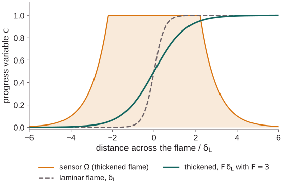
Premixed flames are thinner than LES cells. The dynamically thickened flame
model (TFLES; Colin et al. 2000, Légier et al. 2002) multiplies diffusivities
by E F and reaction rates by E / F inside the flame, so it spans n_res
cells at the right speed; the efficiency E restores the subgrid wrinkling:
by default E = F^beta (Charlette et al. 2002) with beta computed each step
by a dynamic procedure (Wang et al. 2011) from how much resolved flame surface
a test filter removes, so there is no model constant. A sensor Ω confines it to the flame:
[les.combustion]          # examples/flame_turbulence/les.toml: stoichiometric H2/air
model = "tfles"
delta_L = 3.3013976e-4    # laminar thermal thickness [m], from Cantera
s_L = 2.3323744           # laminar flame speed [m/s]
T_unburnt = 300.0
T_burnt = 2384.28
# n_res = 5               # cells across the thickened flame (default)
| Key | Default | Meaning |
|---|---|---|
model |
required | tfles (or the experimental pasr, below) |
delta_L, s_L |
required | Laminar thermal thickness [m] and speed [m/s] |
T_unburnt, T_burnt |
required | Temperatures of fresh and burnt gas [K], for the progress variable |
n_res |
5 | Cells across the thickened flame |
efficiency |
dynamic |
dynamic (E = F^beta, beta from the flow), charlette (efficiency function of a subgrid velocity u') or none (E = 1) |
beta |
0.5 | charlette only: exponent of the efficiency |
subgrid_velocity |
colin |
charlette only: u' of the efficiency, colin or eddy_viscosity (C_u nu_t / Delta) |
C_u |
28 | charlette only: constant of subgrid_velocity = "eddy_viscosity" |
Output: TF_F, TF_E, TF_OMEGA, and tf_beta in the integrals file. Validated on a premixed H2/air flame in
decaying turbulence against its DNS
(validation).
The dynamic efficiency keeps the turbulent flame speed within 8% of two DNS
at cells of 0.4–1.6 delta_L. Pitfalls: beta, subgrid_velocity and C_u
are input errors with dynamic (they belong to charlette); with
charlette, Colin's subgrid velocity doubles the flame speed at 1.6
delta_L; on a nearly flat flame at F = 8 the dynamic E still adds 5–10%.
PaSR (experimental)
model = "pasr": the partially stirred reactor (Sabelnikov & Fureby 2013) for
non-premixed and partially premixed flames. No thickening; each cell's rates
are scaled by its reacting fraction kappa = tau_c / (tau_c + tau_mix),
tau_mix = C_mix Delta^2 / (nu + nu_t) (key C_mix, default 1; output
PASR_KAPPA). It corrects the right way at moderate filter widths and
overcorrects on coarse meshes; validated on one case only
(validation).
Examples
| Example | Shows |
|---|---|
cbc_les |
Decaying isotropic turbulence, Sigma + hybrid flux, 32³ to 128³ |
channel_les |
Wall-resolved channel at Reτ = 395 and 590 |
volvo_bluff_body |
Bluff-body combustor with synthetic inflow and NSCBC outlet |
flame_turbulence |
Premixed flame in turbulence: DNS and TFLES |