Validation

Each result on this page comes from a run of Mallard (double precision, default settings, including the low-Mach correction of the convective flux, unless a section says otherwise), with the inputs described, compared with an exact solution, theory, or published reference data. The line under each heading, and the Version column below, give the release or commit that produced its numbers and figures; later releases change them only where a section says so. Most cases start from an input in Mallard's examples; the scripts that ran every case and drew every figure are in the website repository. Mallard's test suite checks many of the same properties at smaller scale on every change. Mallard 0.5.0 changed two things that affect results: 2D cell centroids are now exact to round-off (#127), which keeps the Sod and Shu–Osher strips one-dimensional (both rerun with 0.5.0) and changes other 2D results at round-off level; and TENO-E ranks stencil candidates by the local mesh spacing on strongly stretched cells (#120), which leaves hexahedral and regular meshes unchanged. Cases marked 3D use Mallard's 3D build (-DMallard_DIM=3); see a 3D case for how to build and run in 3D.

Case	Quantity	Mallard	Reference	Version
Isentropic vortex	order of accuracy, TENO-E orders 3–6	2.99, 4.02, 4.98, 6.03 (quads); 3.00, 4.01, 4.99, 5.99 (triangles)	3, 4, 5, 6	0.3.0
Vortex across a periodic seam	order of accuracy, TENO-E orders 3–6	2.91, 4.08, 4.87, 6.15 (quads); 2.98, 4.03, 4.94, 6.05 (triangles)	3, 4, 5, 6	0.3.0
Curved boundaries	steady vortex between circular walls, L1 rate, TENO-E orders 3–6, curved walls (straight walls do not converge)	3.03, 4.89, 4.90, 4.92	3, 4, 5, 6	0.8.0
Sod shock tube	L1 density error, 200 cells	2.4 × 10−3	exact solution	0.5.0
Shu–Osher problem	L1 density difference, 400 / 800 cells	0.20 / 0.090	WENO5 at 12,800 cells; WENO5 at the same resolution: 0.29 / 0.10	0.5.0
Spherical explosion (3D)	mean density difference, 64³ hexahedra	0.004	1D radial solution, 4000 cells	0.3.0
Sedov–Taylor blast wave (3D)	shock radius error at t = 0.8	+1.1%	exact similarity solution	dev. 0.3.0–0.4.0
Shock–helium bubble (3D)	refracted and transmitted shock, vortex ring, downstream interface velocities	961, 359, 178, 166 m/s	Haas & Sturtevant (1987): 960, 365, 165, 165 m/s	dev. 0.5.0–0.6.0
Oblique shock	shock angle, pressure ratio	42.83°, 1.4985 (TENO-E)	42.82°, 1.4984 (theory)	0.4.0
Mach 3 sphere (3D)	bow-shock standoff Δ/R; stagnation pressure	0.226; 12.0	0.205 (Billig); 12.06 (pitot)	dev. 0.3.0–0.4.0
RHLL on the Mach 3 sphere (3D)	shock on the axis / stagnation pressure, MUSCL, 796k tetrahedra	−0.6151 / 11.93 (before the fix: bulge to −0.624 / 10.6)	HLL: −0.6149 / 11.86	20239fc (in 0.8.0)
Viscous exact solutions	Stokes' first problem: order of accuracy, largest error at 128 rows	second order, 0.0099% of U (quads); order 1.9–2.0, 0.0093% of U (triangles)	exact solution	0.3.0
Viscous shock tube	wall density RMS difference; lambda-shock triple point	0.56 (range 37–118); (0.581, 0.138)	Zhou et al. (2018), 1500 × 750 grid: (0.58, 0.137)	0.4.0
Cylinder, Re = 100	St, mean CD, CL amplitude; with curved walls (384 × 128, TENO3)	0.165, 1.368, 0.331; 0.1648, 1.3629, 0.335	0.164–0.165, 1.33–1.35, 0.33–0.34	not recorded
Sphere, Re = 300 (3D)	St, mean CD, mean CL (2.06M cells)	0.133, 0.666, 0.070	0.134–0.137, 0.655–0.671, 0.065–0.069	dev. 0.3.0–0.4.0
Taylor–Green vortex, Re = 1600 (3D)	peak dissipation rate, at t; largest ε error over t = 0.5–20, of the peak	256³: 0.01289 at 8.83, 3.4%; 128³: 0.01161 at 8.39, 14.1%	512³ spectral DNS: 0.01286 at 8.97	dev. 0.6.0–0.7.0
Compressible isotropic turbulence (3D)	enstrophy, dilatation variance, filtered to 64³, mean over t/τ = 0.2–4, 256³	−2.4%, −0.5%	Johnsen et al. (2010), 256³ filtered	dev. 0.5.0–0.6.0
Channel flow, Reτ = 180 (3D)	Reτ; Cf; peaks of urms, vrms, wrms, −u′v′	180.8; +2.0%; −0.5, +1.8, +1.4, +1.5%	DNS of Moser, Kim & Mansour (1999): 178.1	dev. 0.6.0–0.7.0
Synthetic turbulent inflow (3D)	distance from the inlet to within 5% of the developed channel, all statistics	about 17h	about 20h (Keating et al. 2004)	dev. 0.6.0–0.7.0
0D ignition (reacting)	ignition delay, 36 H2/air and CH4/air mixtures; final temperature	within 3 × 10−6 (H2), 2 × 10−4 (CH4); within 10−5 K	Cantera reactor; Cantera equilibrium	0.4.0
Reactive shock tube (reacting)	reaction front at 230 µs, 50 / 25 / 12.5 µm cells	99.63 / 99.66 / 99.66 mm	converged within one 50 µm cell	0.4.0
CJ detonation (reacting)	front speed; induction length; peak pressure, at 10 / 20 / 40 cells per induction length	+0.11 / +0.01 / 0.00%; −4.5 / −1.8 / +2.7%; 174.8 / 175.2 / 174.7 kPa	DCJ 1616.9 m/s; ZND 1.525 mm; von Neumann 174.7 kPa	0.4.0
Laminar flame speed (reacting)	H2/air, φ = 0.6–1.4, two transport models	within 0.81%	Cantera FreeFlame	0.4.0
Laminar flame speed, CH4/air (reacting)	GRI-3.0, φ = 0.6–1.4, two transport models, 20 cells per thermal thickness	within 1.82%	Cantera FreeFlame	040fb35 (in 0.8.0)
Thermal diffusion (Soret) (reacting)	change of the H2/air flame speed, φ = 0.5 / 1.0	−7.23 / −8.26%	Cantera: −6.98 / −8.44%	caa9b4a (in 0.8.0)
Optically thin radiation (reacting)	Srad/Sad, CH4/air φ = 0.6 / 0.5 (GRI-3.0), 0.44 (two-step)	0.9735 / 0.808 / 0.8507	Cantera: 0.9738 / 0.811 / 0.8509	2d7dde7 (in 0.8.0)
Flame–vortex quenching (reacting, 2D)	outcomes of 12 vortex pairs, r = 1–8 δL, u′ = 3–100 SL	quenching boundary of the shape of the reference's	Poinsot, Veynante & Candel (1991) (qualitative)	2d7dde7 (in 0.8.0)
SIMPLER splitting (reacting)	detonation induction length vs ZND at CFL 1.0, 10 cells; Strang / SIMPLER	−25.5 / −0.9%	ZND 1.525 mm	beb3c3f (in 0.8.0)
Cellular detonation (reacting, 2D)	front speed	1617.0 m/s	DCJ 1616.9 m/s	dev. 0.3.0–0.4.0
Cellular detonation in 3D (reacting)	front speed over 17 cm	1620.6 m/s	DCJ 1617 m/s	dev. 0.5.0–0.6.0
Stratified autoignition (reacting, 2D)	heat release peak time, T′ = 3.75 / 7.5 / 15 / 30 K	0.993 / 0.986 / 0.952 / 0.822 τ0	trend of Chen et al., Hawkes et al. (2006) (qualitative)	dev. 0.5.0–0.6.0
LES, decaying isotropic turbulence (3D)	log10 RMS spectral error at two stations, 128³, Sigma	0.063 / 0.085	Comte-Bellot & Corrsin (1971)	dev. after 0.5.0
LES, channel flow, Reτ = 395 / 590 (3D)	Reτ, Sigma with Scotti's width (64³ / 96³)	+0.7% / +1.6%	392.2 / 587.2 (Moser, Kim & Mansour 1999)	dev. ~0.6.0–0.7.0
LES, bluff-body combustor (3D)	recirculation length Lr/D; εnum/εSGS	1.34; −0.38	1.35 (Sjunnesson et al.)	dev. after 0.6.0 (in 0.8.0)
LES, thickened flame (reacting)	consumption speed at F = 7.9 / 31.6	−0.2% / −0.2%	Cantera sL = 2.3324 m/s	dev. 0.6.0–0.7.0
LES, flame in turbulence (reacting, 3D)	ST/SL, TFLES at Δ = 0.4 / 0.8 / 1.6 δL	1.056 / 1.053 / 2.240	DNS 1.132	dev. 0.6.0–0.7.0
LES, non-premixed flame, PaSR (reacting, 3D, experimental)	heat release, Δ = 0.27 / 0.53 mm	−10.7% / −50% (quasi-laminar +16.6% / +41%)	DNS	dev. 0.6.0–0.7.0

Order of accuracy

Design order on smooth solutions, in 2D, including across periodic seams.

Design-order convergence

Mallard 0.3.0 (0.4.0 changes these errors by at most 0.01%)

The isentropic vortex (Shu 1998) is an exact solution of the Euler equations: a vortex of strength β = 5 in a uniform stream (ρ, u, v, p) = (1, 1, 0.5, 1), γ = 1.4, translating without change of shape. It runs on [0, 14]² from (6.5, 6.75) to t = 1, with the exact moving solution imposed on all four boundaries (dirichlet conditions with expressions in x, y and t), on N × N quadrilaterals and on the same grids split into 2N² triangles, N = 28 to 448. TENO-E of orders 3 to 6, HLLC flux, RK4. The time step is 0.1 h for orders 3 and 4 and 0.1 h (h / h₀)^{(p − 4)/4} for orders p = 5 and 6 (h₀ = 1/2), so that the fourth-order time error falls at least as fast as the spatial error. The error is the area-weighted mean of |ρ − ρ_exact| over all cells, with the exact cell averages from a degree-5 quadrature on 16 sub-triangles of each triangle.

Mean density error of the isentropic vortex at t = 1 against the cell size h (the edge of the quadrilaterals, which the triangles split in two). Dashed lines have slopes 3 to 6.

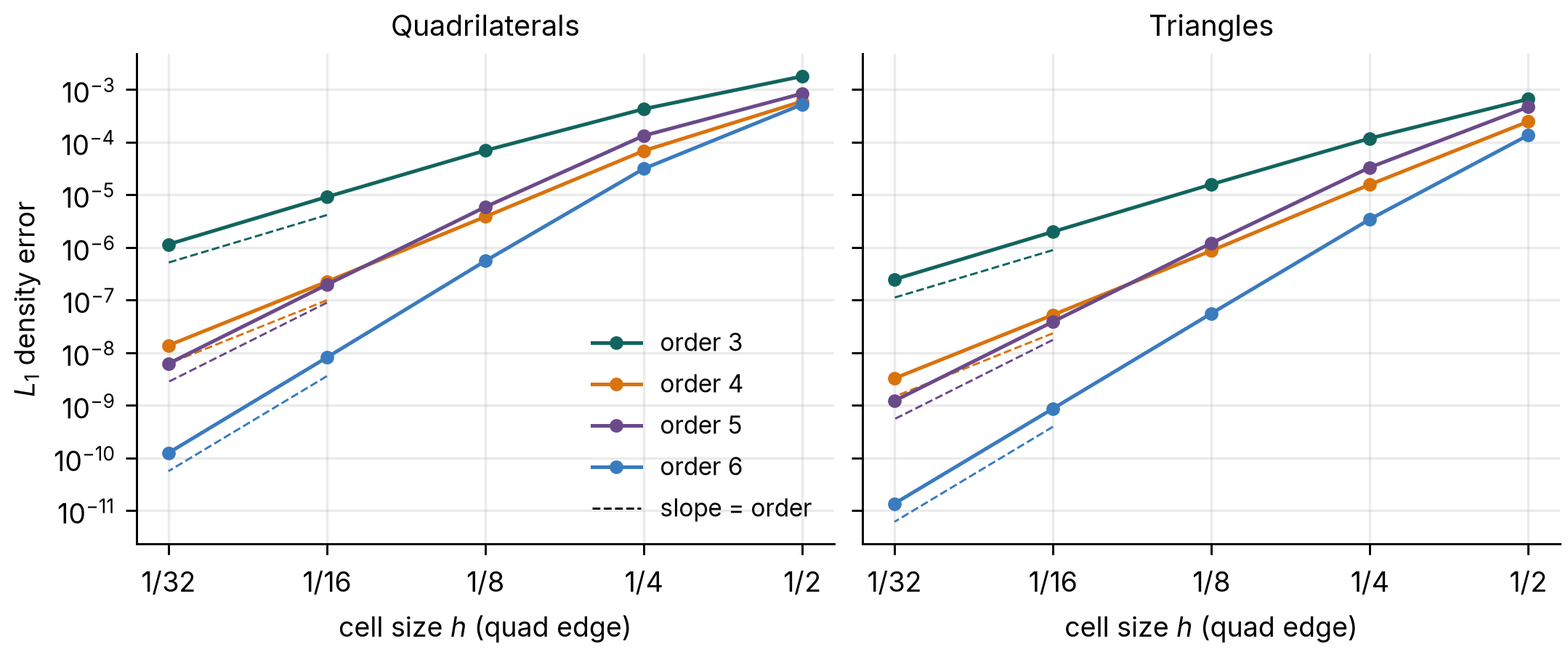
Every order converges at its design rate on both meshes: between the two finest grids the observed orders are 2.99, 4.02, 4.98 and 6.03 on quadrilaterals and 3.00, 4.01, 4.99 and 5.99 on triangles. On the coarsest grids, with only a few cells across the vortex core, the error has not yet reached its asymptotic rate. The maximum error converges at nearly the same rates (2.97 to 6.06 between the two finest grids). Mallard 0.4.0's changes to TENO-E next to boundaries move these errors by at most 0.01% from 0.3.0's.

Quadrilaterals

h	order 3	rate	order 4	rate	order 5	rate	order 6	rate
1/2	1.79 × 10−3		5.99 × 10−4		8.41 × 10−4		5.22 × 10−4
1/4	4.28 × 10−4	2.06	6.88 × 10−5	3.12	1.33 × 10−4	2.66	3.15 × 10−5	4.05
1/8	6.96 × 10−5	2.62	3.85 × 10−6	4.16	5.90 × 10−6	4.50	5.56 × 10−7	5.82
1/16	9.15 × 10−6	2.93	2.24 × 10−7	4.10	1.97 × 10−7	4.90	8.15 × 10−9	6.09
1/32	1.15 × 10−6	2.99	1.38 × 10−8	4.02	6.23 × 10−9	4.98	1.25 × 10−10	6.03

Triangles

h	order 3	rate	order 4	rate	order 5	rate	order 6	rate
1/2	6.61 × 10−4		2.48 × 10−4		4.67 × 10−4		1.36 × 10−4
1/4	1.18 × 10−4	2.48	1.57 × 10−5	3.98	3.32 × 10−5	3.81	3.45 × 10−6	5.30
1/8	1.58 × 10−5	2.90	8.70 × 10−7	4.17	1.21 × 10−6	4.78	5.59 × 10−8	5.95
1/16	1.99 × 10−6	2.99	5.24 × 10−8	4.05	3.89 × 10−8	4.96	8.69 × 10−10	6.01
1/32	2.48 × 10−7	3.00	3.26 × 10−9	4.01	1.22 × 10−9	4.99	1.36 × 10−11	5.99

Across periodic seams

Mallard 0.3.0 (0.4.0 gives the same errors to seven digits)

Mallard 0.3.0 makes generated meshes periodic ([mesh] periodic = ["x", "y"]): the faces on opposite sides of the box become interior faces, and every stencil reaches across them. To check that the seam costs no accuracy, the same vortex runs in the doubly periodic box [0, 14]², starting centered 1 unit inside the right edge, so that it straddles the seam, and moving with (u, v) = (1, 0) to t = 2, through the seam to the other side. Initial data and the exact solution use the nearest periodic image; everything else is as above, on N = 28 to 224.

Between the two finest grids the observed orders are 2.91, 4.08, 4.87 and 6.15 on quadrilaterals and 2.98, 4.03, 4.94 and 6.05 on triangles: the design orders, as without the seam. Without boundaries, these runs are not affected by 0.4.0's changes to TENO-E next to walls: the errors are those of 0.3.0 to seven digits. Since 0.4.0, meshes read from Gmsh files can be periodic too, by pairing boundary zones in [[periodic]] tables.

Quadrilaterals, periodic

h	order 3	rate	order 4	rate	order 5	rate	order 6	rate
1/2	2.80 × 10−3		7.15 × 10−4		1.22 × 10−3		6.54 × 10−4
1/4	5.72 × 10−4	2.29	8.29 × 10−5	3.11	1.62 × 10−4	2.92	4.25 × 10−5	3.95
1/8	9.34 × 10−5	2.61	4.82 × 10−6	4.10	8.23 × 10−6	4.30	8.96 × 10−7	5.57
1/16	1.24 × 10−5	2.91	2.85 × 10−7	4.08	2.82 × 10−7	4.87	1.26 × 10−8	6.15

Triangles, periodic

h	order 3	rate	order 4	rate	order 5	rate	order 6	rate
1/2	9.19 × 10−4		2.95 × 10−4		5.37 × 10−4		1.71 × 10−4
1/4	1.59 × 10−4	2.53	2.01 × 10−5	3.87	4.65 × 10−5	3.53	5.17 × 10−6	5.05
1/8	2.19 × 10−5	2.86	1.16 × 10−6	4.11	1.85 × 10−6	4.65	8.41 × 10−8	5.94
1/16	2.77 × 10−6	2.98	7.14 × 10−8	4.03	6.06 × 10−8	4.94	1.27 × 10−9	6.05

Curved boundaries

Mallard 0.8.0 (177818c, merge of #263)

Since 0.8.0, faces on curved walls follow the true geometry to the order of the scheme (guide). The geometry comes from high-order Gmsh boundary elements, or from an analytic projection onto circles and spheres. Straight-sided cells next to a curved wall misplace it by O(h²/R): that error enters the face quadrature points, the normals, and every moment TENO-E fits. At slip walls the polygonal wall also turns the flow at every node.

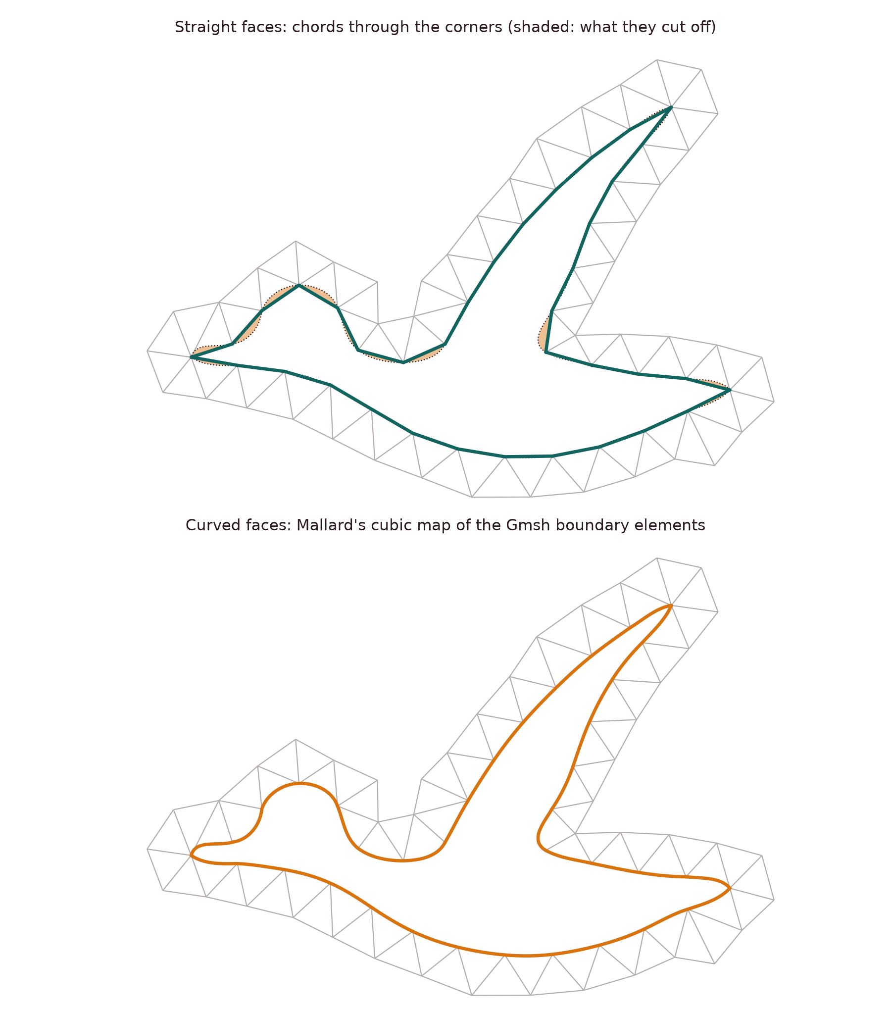
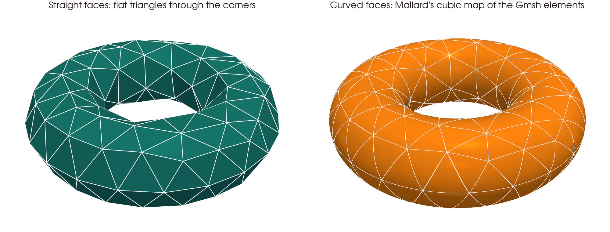
Mallard keeps the corners of every cell and curves the faces on the wall. The figures below show this on coarse Gmsh meshes with cubic boundary elements, whose extra nodes Gmsh places on the geometry. The straight panels show the faces through the corners, as with [mesh] curved_geometry = false. The curved panels show Mallard's face map, the cubic through each boundary element's nodes, sampled finely.

The outline of the `mallard` example, meshed with triangles of size 0.1 (36 faces on the wall); only the triangles touching the wall are drawn. Top: chords through the corners, with the area they cut off shaded. Bottom: the curved faces.

A torus meshed with 266 cubic triangles. Left: flat triangles through the corners. Right: the same faces through Mallard's cubic map, with their edges along it.

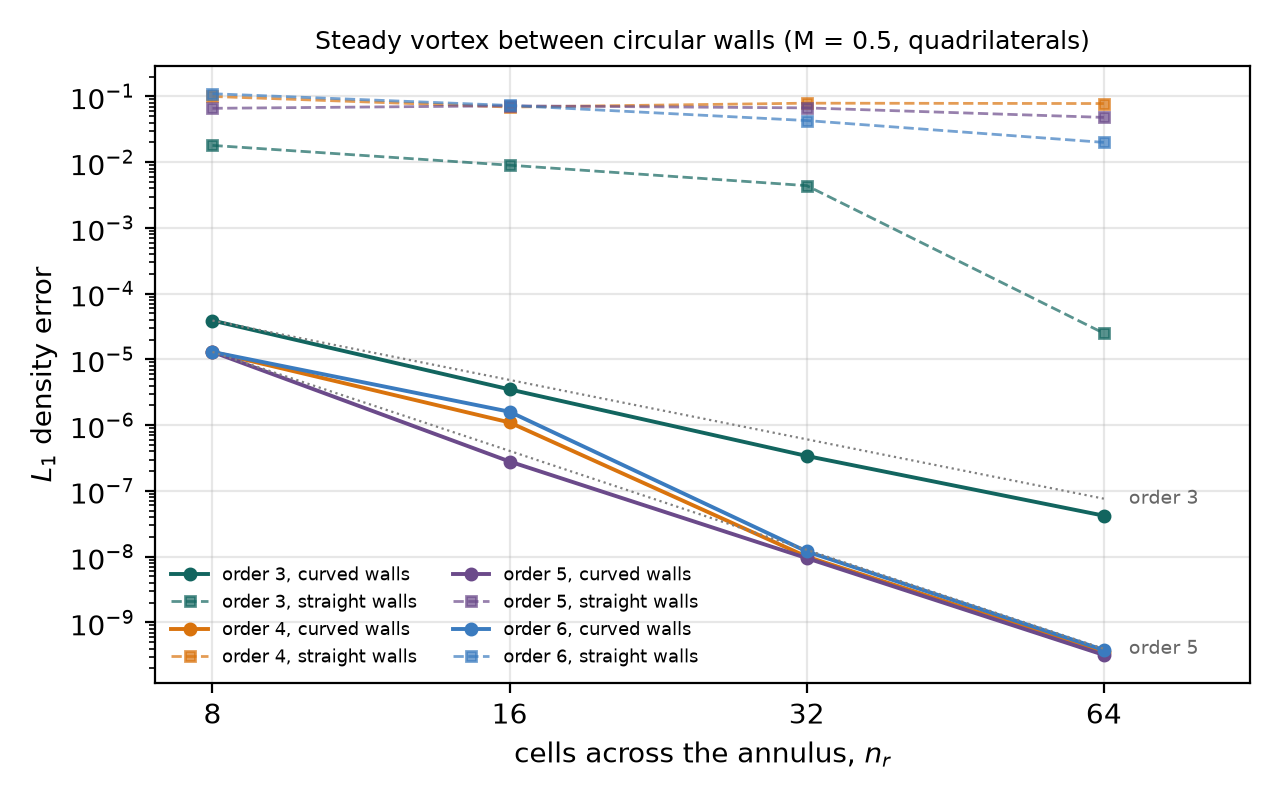
The test case is the irrotational vortex u_θ = M/r in the annulus 1 ≤ r ≤ 1.384, an exact steady Euler solution with slip walls on both circles. It runs on quadrilateral O-grids of n_r × 16 n_r cells (triangles: each split in two), HLLC, SSPRK3 at CFL 0.4, from the exact cell averages to t = 12. The error is the L₁ density error against the exact averages.

Subsonic vortex (M = 0.5) on quadrilaterals: with curved walls every order converges; with straight walls none does.

TENO-E order	3	4	5	6
L1 rate, subsonic, quadrilaterals, curved	3.03	4.89	4.90	4.92
L1 at nr = 64, curved / straight	4.2 × 10−8 / 2.5 × 10−5	3.5 × 10−10 / 7.8 × 10−2	3.2 × 10−10 / 4.8 × 10−2	3.8 × 10−10 / 2.0 × 10−2
L∞ rate, subsonic, quadrilaterals, curved	2.86	3.99	3.95	3.65
L1 rate, subsonic, triangles, curved	3.45	4.38	4.91	4.91
L1 rate, supersonic (M = 2.25), quadrilaterals, curved	3.64	4.86	5.00	5.57

• Straight walls: no order converges. The subsonic L₁ errors at n_r = 64 are 2 × 10⁻² to 8 × 10⁻² for orders 4–6. The supersonic vortex sheds waves at every node, with errors of 0.05 to 0.26.
• Order at the wall: orders 5 and 6 converge at fourth order. The central fits of cells reaching a curved wall are capped at degree 3, because one-sided degree-4 and -5 fits grow exponentially there; design order needs a boundary-constrained reconstruction.
• Gmsh geometry: P3 walls from a Gmsh file (line4) match the analytically projected walls to three digits.
• Applications: the cylinder and the Mach 3 sphere with curved walls are in their own sections.

Shock tubes and blast waves

Discontinuous solutions against exact or converged references, in 1D strips, 2D and 3D.

Sod shock tube

Mallard 0.5.0

The Riemann problem of Sod (1978): (ρ, u, p) = (1, 0, 1) for x < 0.5 and (0.125, 0, 0.1) for x > 0.5, γ = 1.4, at t = 0.2. The sod example: a strip of N × 4 square quadrilaterals with slip walls, HLLC flux, SSPRK3 at CFL 0.5. Run with Mallard 0.5.0.

Sod shock tube at t = 0.2 on 200 cells. Fifth-order TENO-E (dots) and MUSCL with the Venkatakrishnan limiter (line) against the exact solution.

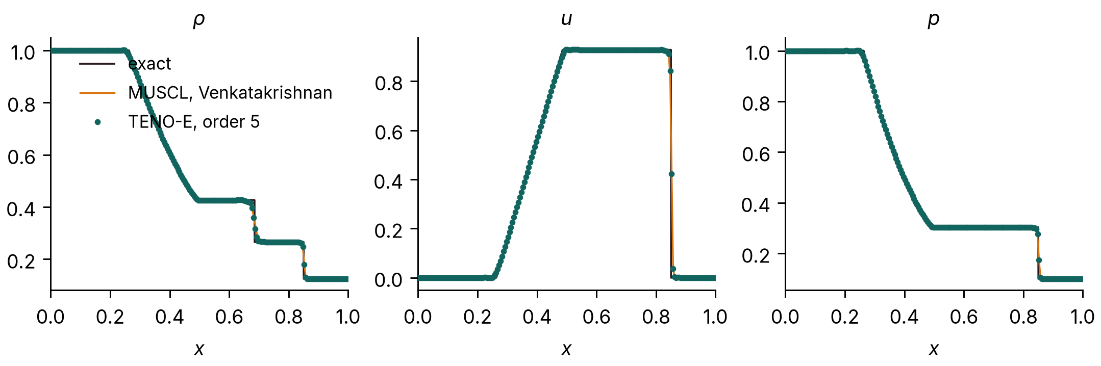
L₁ error of the cell-averaged density, ∫|ρ − ρ_exact| dx, with the exact solution averaged over each cell, over all cells of the strip:

Cells	TENO-E 5	rate	MUSCL	rate
100	4.16 × 10−3		4.46 × 10−3
200	2.41 × 10−3	0.79	2.65 × 10−3	0.75
400	1.27 × 10−3	0.93	1.43 × 10−3	0.89
800	6.65 × 10−4	0.93	7.65 × 10−4	0.90

Both schemes converge at close to first order, the expected rate for a solution with a shock and a contact discontinuity; TENO-E has 7–13% lower error than MUSCL. The shock spans two cells and the contact discontinuity about five.

The errors are taken over all cells of the strip, whose four rows agree to round-off (5 × 10⁻¹⁴) at every resolution with Mallard 0.5.0. In 0.3.0 the rows next to the slip walls differed from the inner two, and the errors quoted here were those of the bottom row (3.92, 2.28, 1.21 and 0.60 × 10⁻³ for TENO-E); in 0.4.0 the TENO-E rows differed by up to 5 × 10⁻³ on 800 cells (error 7.24 × 10⁻⁴). MUSCL results are the same in all three versions.

Sod shock tube in 3D

Text: Mallard 0.3.0. Figure and table: rerun with Mallard 0.7.0

The Sod problem of the Sod shock tube section on a 200 × 4 × 4 box of hexahedra with slip walls on all six faces, MUSCL with the Venkatakrishnan limiter, HLLC, SSPRK3. The solution stays one-dimensional to round-off (transverse velocities below 10⁻¹³), and its L₁ density error against the exact solution, 2.653 × 10⁻³, equals that of the same scheme on 200 × 4 quadrilaterals in 2D to all four digits.

Every one of the 200 × 4 × 4 cells at t = 0.2 (MUSCL with the Venkatakrishnan limiter, HLLC), against the exact solution; Mallard 0.7.0.

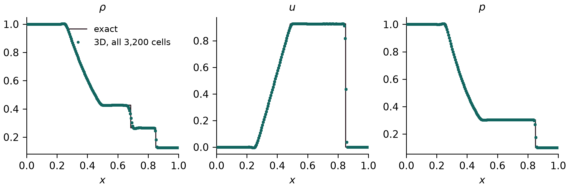
Run	L1 density error	largest transverse velocity	largest density spread across a cross-section
3D, 200 × 4 × 4 hexahedra, Mallard 0.7.0	2.662 × 10−3	1.5 × 10−14	3.4 × 10−14
3D, the same, Mallard 0.3.0	2.653 × 10−3	below 10−13
2D, 200 × 4 quadrilaterals, Mallard 0.5.0 (table above)	2.65 × 10−3

The 0.7.0 rerun uses the sod example's settings in 0.7.0 (CFL 1.0 in that release's time-step convention, #175); the solution stays one-dimensional to round-off.

Shu–Osher problem

Mallard 0.5.0

A Mach 3 shock running into a sinusoidal density field (Shu & Osher 1989), on [0, 10] (the usual [−5, 5] shifted by 5), t = 1.8, with the shu_osher example: fifth-order TENO-E and the RHLL flux on N × 4 square quadrilaterals, run with Mallard 0.5.0. There is no exact solution; the reference is a one-dimensional fifth-order WENO-JS solution (characteristic, Lax–Friedrichs flux splitting, SSPRK3) on 12,800 cells, which differs from the same code on 6,400 cells by 0.007 in L₁.

Shu–Osher problem at t = 1.8: fifth-order TENO-E with the RHLL flux on 200 and 400 cells against the 12,800-cell reference. Right: the entropy waves generated behind the shock, the part of the solution that separates high-order schemes.

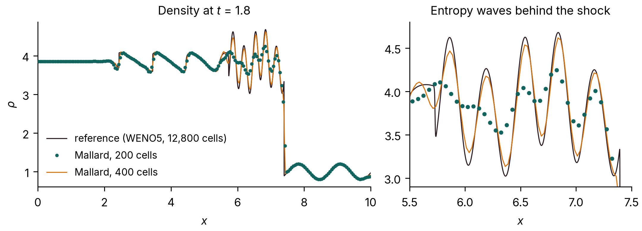
L₁ density difference from the reference, ∫|ρ − ρ_ref| dx:

Cells	Mallard, RHLL	Mallard, HLLC	1D WENO5, same cells
200	0.66	0.65	0.75
400	0.20	0.21	0.29
800	0.090	0.31	0.10
1600	0.043	0.65	0.048

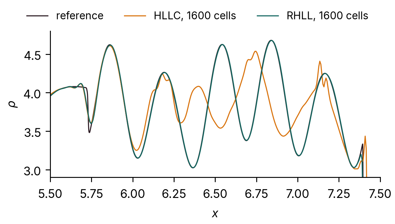
With the rotated-hybrid RHLL flux, Mallard converges to the reference and is more accurate than the one-dimensional WENO5 scheme on every grid (0.3.0 had 0.26, 0.12 and 0.082 on 400, 800 and 1600 cells; 0.4.0 0.20, 0.11 and 0.059). With HLLC it does not converge beyond 400 cells: behind the Mach 3 shock, which moves along the grid lines of the strip, the rows of a problem that should stay one-dimensional differ by up to 1.1 in density on 800 and 1600 cells, and the entropy waves are lost. This is the grid-aligned shock instability that Quirk (1994) described for Roe's scheme and to which HLLC is also prone; use RHLL for strong shocks aligned with quadrilateral grids. The example has used RHLL since Mallard 0.3.0 (0.2.0's used HLLC). With RHLL the rows differ by up to 0.07 on 800 cells and 10⁻⁵ on 1600.

Entropy waves on 1600 cells with the HLLC and RHLL fluxes.

Spherical explosion (3D)

Mallard 0.3.0 (0.4.0 reproduces it bit for bit)

The spherical explosion of Toro (Riemann Solvers and Numerical Methods for Fluid Dynamics, 3rd ed., §17.1.3), the explosion_3d example: a sphere of radius 0.4 at ρ = 1, p = 1 in a gas at ρ = 0.125, p = 0.1, run to t = 0.25. One octant, [0, 1]³, is computed on 64³ hexahedra with symmetry planes at x, y, z = 0 and transmissive outer faces; fifth-order TENO-E, HLLC, SSPRK3. The reference is a solution of the radial Euler equations (fifth-order WENO on 4000 cells), from the validation scripts.

Density at t = 0.25 of all 262,144 cells against their distance from the center, and the radial reference: the rarefaction running into the center, the contact near r = 0.6 and the shock near r = 0.8.

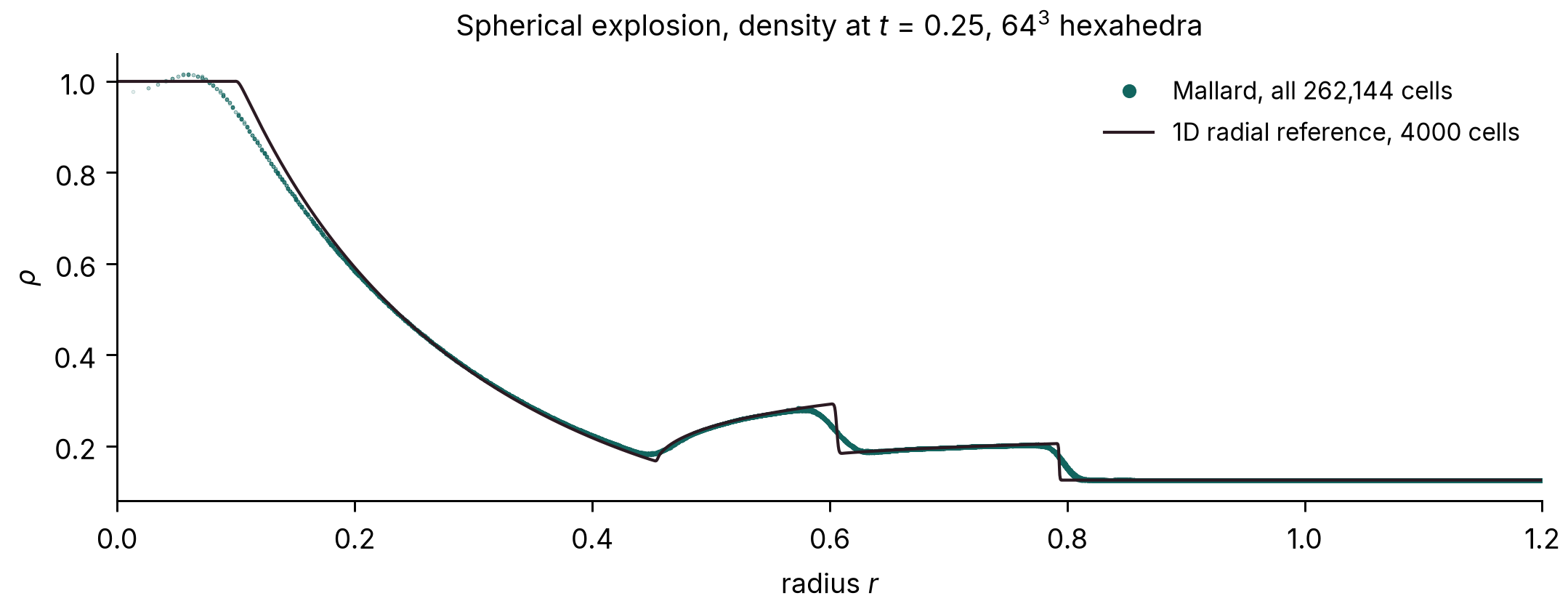
The cells collapse onto one curve, so the computed flow stays spherically symmetric on the Cartesian mesh, and that curve follows the reference: the mean absolute difference in density is 0.004 (cells with r < 0.95), most of it at the discontinuities, which the 64³ mesh spreads over two to three cells. Mallard 0.4.0 reproduces the 0.3.0 run bit for bit.

Sedov–Taylor blast wave (3D)

Development code between 0.3.0 and 0.4.0 (commit not recorded; 0.4.0 is bitwise the same on hexahedra)

A point explosion in a gas at rest (Taylor 1950; Sedov 1959), the sedov_3d example (new in Mallard 0.4.0): the energy is deposited in a small sphere at the origin, and only the octant x, y, z ≥ 0 is computed, with three symmetry planes, on 128³ hexahedra (2,097,152 cells); fifth-order TENO-E with bound-preserving scaling, HLLC, SSPRK3, to t = 0.8, on A100 GPUs, run with the development code between 0.3.0 and 0.4.0 (0.4.0's changes to TENO-E leave results on hexahedra bitwise the same). The exact similarity solution for γ = 1.4 puts the shock at R = ξ₀(E t²/ρ₀)^1/5 with ξ₀ = 1.0328.

Density on the three symmetry planes, the shock radius against the similarity solution, and the density of the cells on the planes against the exact profile.

t	0.1	0.2	0.4	0.6	0.8
Shock radius, error against the similarity solution	+2.6%	+1.9%	+1.5%	+1.2%	+1.1%

The shock-radius error decays as the run forgets the finite radius of the initial blast. The density profile follows the exact curve, with the peak behind the shock smeared to 4.2 (averaged over the shell) against 6 at this resolution, and varies by 2.5% over the shell at the peak; mass is conserved to round-off.

Shock–helium bubble interaction (3D)

Development code between 0.5.0 and 0.6.0: 3bec90f with the tools of #183

A Mach 1.25 shock in air hits a helium bubble, the spherical case of Haas & Sturtevant (1987), in the shock_bubble_3d example. Navier–Stokes with mixture-averaged transport in He + N₂/O₂; the bubble holds 28% air, which gives a sound speed of 871.5 m/s (Haas & Sturtevant estimate 872). The gases, Mach number and tube are the experiment's in units of the bubble diameter D, but the bubble is scaled down to 0.18 mm, so Re = 1.5 × 10³ instead of 3 × 10⁵. The domain is a quarter of the square tube with symmetry planes, at 128 cells per D: 11.4 million hexahedra. The run took 52,091 steps, 3.4 hours on four A100 GPUs.

The helium surface (Y = 0.15), and the vortex sheet and ring colored by helium fraction; numerical schlieren on the symmetry plane; positions on the axis against the measured velocities. Times and lengths at the experiment's scale.

Velocity [m/s]	Mallard, 128 cells per D	Haas & Sturtevant
refracted shock	961	960
transmitted shock	359	365
vortex ring	178	165
downstream interface, late	166	165

All four are within 0–8% of the measurements, inside their 10% uncertainty, and within 1.2% of a run at 96 cells per D. The upstream interface, the air jet and the late upstream face move differently from the experiment. At this Reynolds number and a Péclet number of about 190, the trailing helium is drawn into the ring.

Shocks on bodies

Oblique shock (2D)

Mallard 0.4.0 (MUSCL unchanged from 0.3.0)

Mach 1.758 flow (u = 600 m/s, T = 300 K, R = 277.4 J/(kg K)) over an 8° compression ramp, the wedge example: 160 × 120 quadrilaterals, HLLC, SSPRK3, run to t = 0.02 s (six flow-through times). The oblique-shock relations give a shock angle β = 42.816° and a pressure ratio p₂/p₁ = 1.4984. The measured angle is a straight-line fit to the half-jump pressure contour for 0.7 < x < 1.6 m; the pressure ratio is the mean over the cells 0.03–0.12 m above the ramp for 0.9 < x < 1.1 m.

Left: pressure with the theoretical shock (dashed). Right: pressure across the shock at x = 1.51 m with MUSCL and fifth-order TENO-E against the theoretical jump.

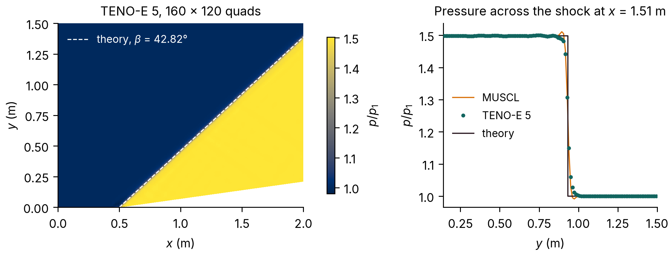
Source	Shock angle	Error	p2/p1	Error
Theory	42.816°		1.4984
MUSCL	42.814°	−0.002°	1.4984	< 0.01%
TENO-E 5	42.826°	+0.011°	1.4985	+0.01%

The fitted shock passes through x = 0.4997 m at y = 0, the ramp corner being at x = 0.5 m. MUSCL results are unchanged from Mallard 0.3.0; with 0.4.0's TENO-E changes next to walls, the TENO-E shock angle moved from 42.821° to 42.826°.

Mach 3 flow over a sphere (3D)

Development code between 0.3.0 and 0.4.0, before #109 (commit not recorded)

Inviscid Mach 3 flow past a sphere of diameter D, started impulsively, the sphere_mach3 example (new in Mallard 0.4.0): 796,962 tetrahedra in the quarter domain y, z ≥ 0 with two symmetry planes, refined on the sphere and through the shock layer; fifth-order TENO-E with bound-preserving scaling, HLL flux, SSPRK3, to t u_∞/D = 3, on 4 GPUs. HLL rather than RHLL, because RHLL develops a carbuncle on the axis where the two symmetry planes meet (issue #80). This run used the development code before two 0.4.0 changes to TENO-E, the conditioning bound and complete stencils near boundaries (#109), which change results on tetrahedra; it has not been repeated with 0.4.0.

Mach number on the horizontal meridian, numerical schlieren on the vertical one and the revolved bow shock; the shock standoff distance against Billig's correlation, and the pressure along the stagnation line.

	Mallard	Reference
Shock standoff Δ/R	0.226	0.205 (Billig 1967 correlation)
Stagnation pressure p0/p∞	12.0	12.06 (Rayleigh pitot formula)
Pressure drag coefficient	0.95

The standoff is steady from t u_∞/D ≈ 1.2. It is 10% above Billig's empirical correlation, a difference of 0.01 D, under half the 0.025 D edge of the tetrahedra in the shock layer.

With curved walls (Mallard 0.8.0, 177818c): the same flow on 810,000 tetrahedra in a quarter box (the faceted quarter-cylinder far field above exceeds the 3D setup's 32 mirror planes with curved walls), at t u_∞/D = 3.

Scheme	Walls	Δ/R (Billig 0.205)	pressure CD
MUSCL	straight	0.2211	0.9716
MUSCL	curved	0.2212	0.9720
TENO5, bound-preserving	curved	0.2213	0.9790

With 0.02 D cells on the wall the facets sit 10⁻⁴ D inside the sphere, so the standoff does not move. TENO5 with straight walls cannot run on this mesh: the sphere's facets are mirror planes of their own, beyond the setup's limit.

RHLL on the Mach 3 sphere

20239fc (merge of #248); first released in Mallard 0.8.0

With MUSCL on tetrahedra, the rotated-hybrid RHLL flux grew a carbuncle on the bow shock. On faces that cross the shock at an angle, its rotation turned the HLL part onto the shock normal instead of the face normal. Since #248, RHLL blends the rotated flux toward HLL along the face normal by the pressure jump across the face, w = min(p_l/p_r, p_r/p_l)³. Contacts and shear layers have no pressure jump, so they keep the rotated flux. Inviscid Mach 3 flow over the sphere with MUSCL, at t = 2, gives the shock position on the axis and the stagnation pressure:

Mesh	RHLL before the fix	RHLL with the fix	HLL
quarter sphere, 121k tetrahedra	carbuncle: −0.687 / 9.0 at t = 1.2	−0.6086 / 11.62	−0.6087 / 11.71
full sphere, 475k tetrahedra	−0.630 / 9.1	−0.6163 / 12.04	−0.6163 / 12.11
example mesh, 796k tetrahedra (quarter)	bulges to −0.624 / 10.6 at t = 1.2–1.4	−0.6151 / 11.93, steady	−0.6149 / 11.86

With the fix, RHLL matches HLL's shock position to 10⁻⁴ D. With TENO5 on the example mesh it gives −0.6157 to t = 1.8, as before the fix. Results of the other Riemann solvers are unchanged.

Viscous flow

Viscous exact solutions

Mallard 0.3.0

Three exact solutions of the compressible Navier–Stokes equations in a channel 0 < y < 1, computed on strips 0.25 wide of N/4 × N square cells (quadrilaterals, or the same split into triangles) with transmissive ends, μ constant, Pr = 0.72, R = 1, γ = 1.4, MUSCL reconstruction (Venkatakrishnan limiter), HLLC, SSPRK3 at CFL 0.8:

• Couette flow: a wall at rest at y = 0 and a wall moving at U = 0.1 at y = 1, both isothermal at T = 1, μ = 0.2, run to steady state (t = 15). Exact: u = U y.
• Stokes' first problem: a wall started impulsively at U = 0.05 under fluid at rest, ν = 0.01, a symmetry plane at y = 1, t = 2. Exact: u = U erfc(y / 2√(νt)).
• Conduction: walls at rest at T = 1.2 and T = 0.8, μ = 0.2, steady state (t = 20). Exact: T = 1.2 − 0.4 y.

Couette flow and conduction on 16 rows of cells, Stokes' first problem on 32 rows, against the exact solutions.

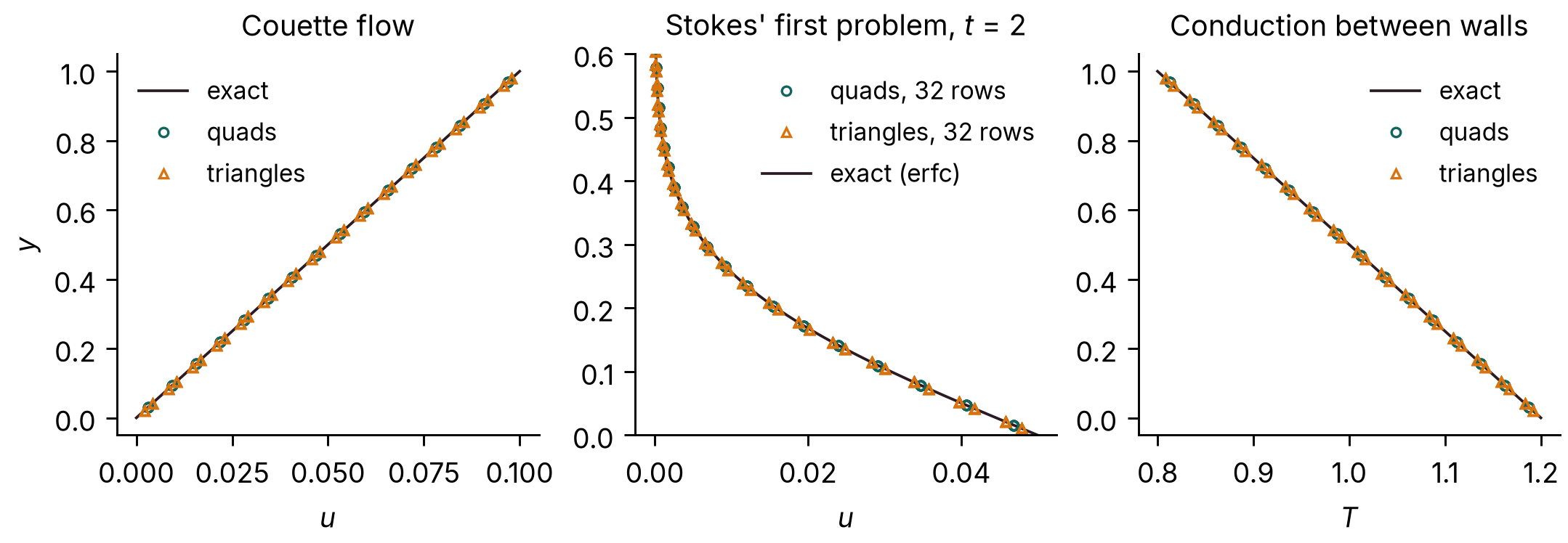
On quadrilaterals the linear Couette and conduction profiles are reproduced to round-off (largest error 1e-13 of U and 5e-14 of the temperature difference); on triangles the largest errors are 7.44 × 10⁻⁷ of U and 1.03 × 10⁻⁵ of the temperature difference. For Stokes' first problem, the largest velocity error relative to U:

Rows	Quadrilaterals	rate	Triangles	rate
16	6.56 × 10−3		5.19 × 10−3
32	1.58 × 10−3	2.05	1.38 × 10−3	1.92
64	3.97 × 10−4	2.00	3.51 × 10−4	1.97
128	9.94 × 10−5	2.00	9.27 × 10−5	1.92

The viscous terms converge at second order on quadrilaterals and at 1.9 to 2.0 on these right triangles (0.0093% of U at 128 rows). With Mallard 0.2.0, on strips only 4 cells wide, the triangle error stalled near 0.4% of U. That came from the transmissive ends of the strip, not from the interior scheme: the viscous fluxes on triangles next to transmissive boundaries, which Mallard 0.3.0 makes second-order, and a one-sided gradient at those ends, which dominates when the strip narrows with refinement. The strip now keeps a fixed width of 0.25.

Viscous shock tube (2D)

Mallard 0.4.0

The viscous shock tube of Daru & Tenaud (2009) at Re = 200: a diaphragm at x = 0.5 in a closed unit box releases a Mach 2.37 shock (density ratio 100) that reflects off the end wall and interacts with the boundary layer it has laid down on the floor, forming a lambda shock and a primary vortex by t = 1. The viscous_shock_tube example computes the lower half, [0, 1] × [0, 0.5], on 1000 × 500 quadrilaterals with no-slip adiabatic walls and a symmetry plane on top; Navier–Stokes, Pr = 0.73, fifth-order TENO-E, HLLC, SSPRK3 at CFL 0.8 (about 58,500 time steps, limited by viscosity). The reference is the grid-converged solution of Zhou et al. (2018) on 1500 × 750 cells.

Viscous shock tube at t = 1 on 1000 × 500 quadrilaterals. Top: density near the floor with the reference triple point and primary-vortex height. Bottom: density in the first row of cells against the tabulated wall density of Zhou et al. (2018).

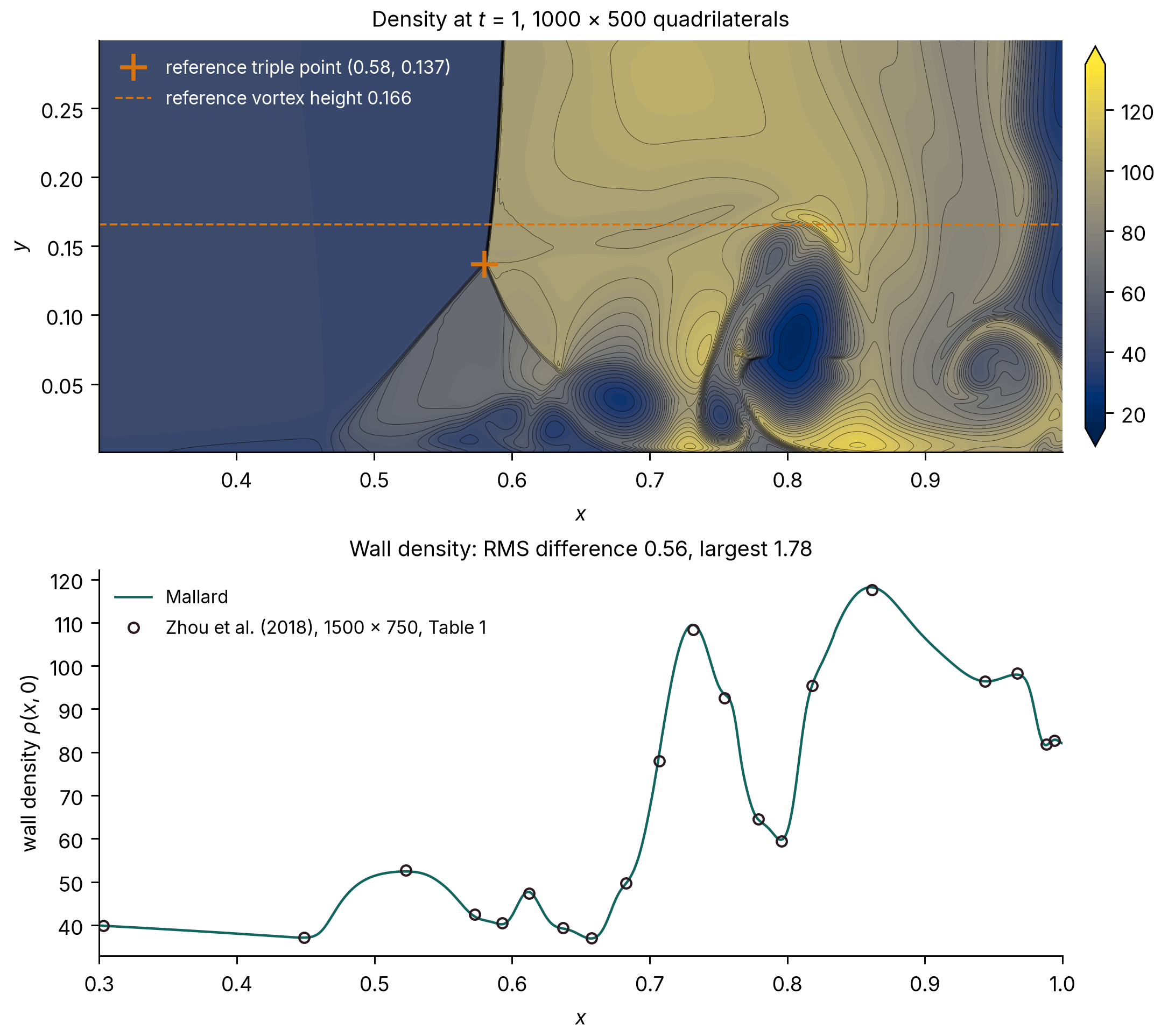
Quantity	Mallard, 1000 × 500	Zhou et al., 1500 × 750 (Table 1)
Lambda-shock triple point (x, y)	(0.581, 0.138)	(0.58, 0.137)
Wall density minimum, at x	36.90, 0.6575	36.96, 0.6577
Wall density maximum, at x	118.19, 0.8605	117.65, 0.8617
Wall density, RMS difference at the 20 tabulated points	0.56
Wall density, largest difference	1.78 (at x = 0.707, on the steep rise to the second peak)

The triple point is the intersection of straight-line fits to the density-gradient ridges of the lambda's front leg and the reflected shock above it. The wall density varies from 37 to 118 along the floor, so the RMS difference is 0.7% of that range. On a mesh coarsened by a factor of two in each direction (500 × 250) the RMS difference is 2.21, the largest 7.33, and the triple point is at (0.580, 0.140): the solution converges toward the reference with the mesh.

Cylinder at Re = 100 (2D)

Version not recorded: rerun with Mallard 0.3.0, with the force amplitudes and figures updated at the 0.5.0 site update

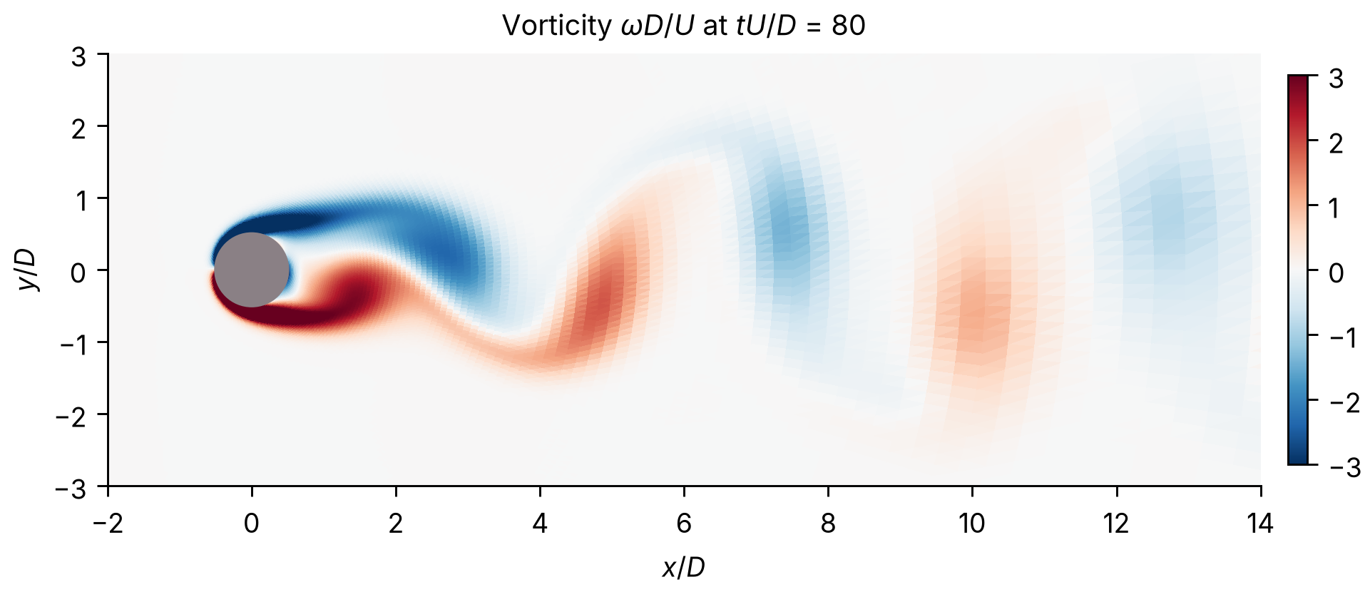
Viscous flow past a circular cylinder at Re = U D / ν = 100 and Mach 0.2, the cylinder example: an O-grid of 384 × 128 quadrilaterals reaching 25 D, first cell 0.01 D, generated with tools/make_cylinder_mesh.py. Adiabatic no-slip wall, characteristic far field, third-order TENO-E, HLLC, SSPRK3 at CFL 0.8, run to t U / D = 80. Shedding is fully developed by t U / D = 12, and the statistics are taken over the ten complete lift cycles after that.

Vorticity at t U / D = 80.

Drag and lift on both meshes, with the averaging window shaded and the means of Johnson & Patel (1999) dashed; the finer run starts from the coarser at t U / D ≈ 49.

Left: drag and lift coefficients. Right: Strouhal number, mean drag and lift amplitude relative to Liu et al. (1998).

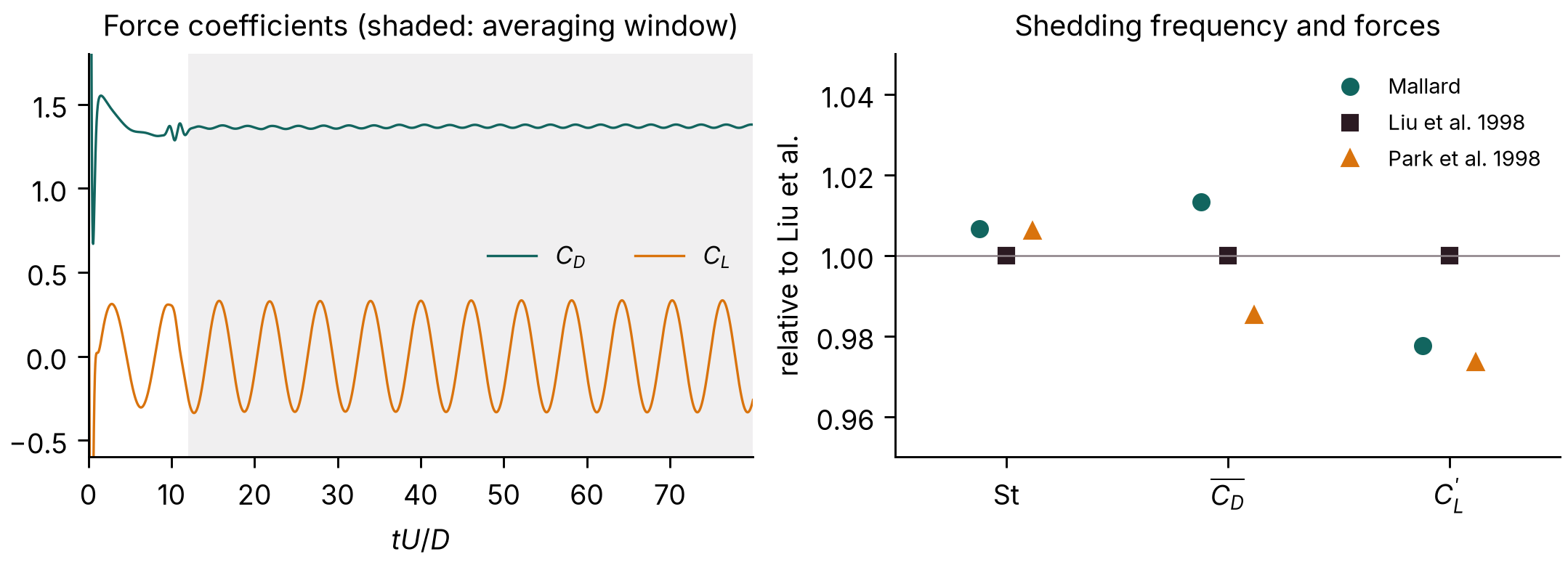
Source	St	mean CD	CD amplitude	CL amplitude
Mallard, 384 × 128	0.1651	1.368	0.014	0.331
Mallard, 768 × 256, first cell 0.005 D	0.1651	1.365	0.015	0.330
Liu, Zheng & Sung (1998)	0.164	1.350	0.012	0.339
Park, Kwon & Choi (1998)	0.165	1.33		0.33
Williamson (1996), experiment	0.164

The references are incompressible computations (Liu et al., Park et al.) and experiments (Williamson); Mallard's run is compressible at Mach 0.2. On a mesh refined by a factor of two in each direction (768 × 256 cells, first cell 0.005 D, run to t U / D = 60: seven lift cycles) the Strouhal number does not change (to 0.01%), and the mean drag and lift amplitude change by 0.2% and 0.4%.

With curved walls (Mallard 0.8.0, 177818c): examples/cylinder with the wall and the far field curved, statistics over t U/D = 60–160.

Mesh	Order	Walls	St	mean CD	CL amplitude
128 × 64	3	straight	0.1633	1.3671	0.335
128 × 64	3	curved	0.1633	1.3643	0.337
128 × 64	5	straight	0.1647	1.3698	0.335
128 × 64	5	curved	0.1647	1.3656	0.333
384 × 128	3	straight	0.1648	1.3637	0.334
384 × 128	3	curved	0.1648	1.3629	0.335
384 × 128	5	straight	unstable	1.349 (fluctuations ±2.9)	2.76
384 × 128	5	curved	0.1648	1.3614	0.331

At Re = 100 the boundary layer spans many cells, so curving the wall moves the drag by only 0.1–0.3%, toward the incompressible 1.33–1.35. On the fine mesh, fifth-order TENO-E with straight walls is unstable; with curved walls it runs.

Sphere at Re = 300 (3D)

Forces: development code before 0.4.0, with 0.4.0's MUSCL (#111; commit not recorded). Animation: rerun between 0.5.0 and 0.6.0 for #139

Viscous flow past a sphere at Re = U D / ν = 300 and Mach 0.2, the sphere_re300 example (new in Mallard 0.4.0; run with 0.4.0's MUSCL, whose gradients on tetrahedra use vertex neighbours, #111). At this Reynolds number the wake sheds hairpin vortices periodically and keeps one plane of symmetry, so the sphere feels a mean lift as well as drag (Johnson & Patel 1999). The mesh, from tools/make_sphere_re300_mesh.py, has 10 layers of prisms on the sphere, from 0.005 D, and tetrahedra refined through the near wake, on the full box −15 < x/D < 30, |y|, |z| < 15. Navier–Stokes, MUSCL with HLLC, SSPRK3 at CFL 0.8; MUSCL rather than TENO-E, which is currently unstable on the thin boundary-layer prisms. The coefficients are averaged over the 7 shedding periods of t U / D = 90–150; the 0.85M-cell run took 4.7 h on 4 A100 GPUs, and the 2.06M-cell one, refined by 1.4 in every direction, 6.7 h on 8.

Q-criterion isosurfaces colored by streamwise velocity, and the drag and lift coefficients over time.

	St	mean CD	mean CL
Mallard, 0.85M cells	0.1331	0.6688	0.0731
Mallard, 2.06M cells	0.1328	0.6664	0.0697
Johnson & Patel (1999)	0.137	0.656	0.069
Kim, Kim & Choi (2001)	0.134	0.657	0.067
Constantinescu & Squires (2003)	0.136	0.655	0.065
Tomboulides, Orszag & Karniadakis (1993)	0.136	0.671

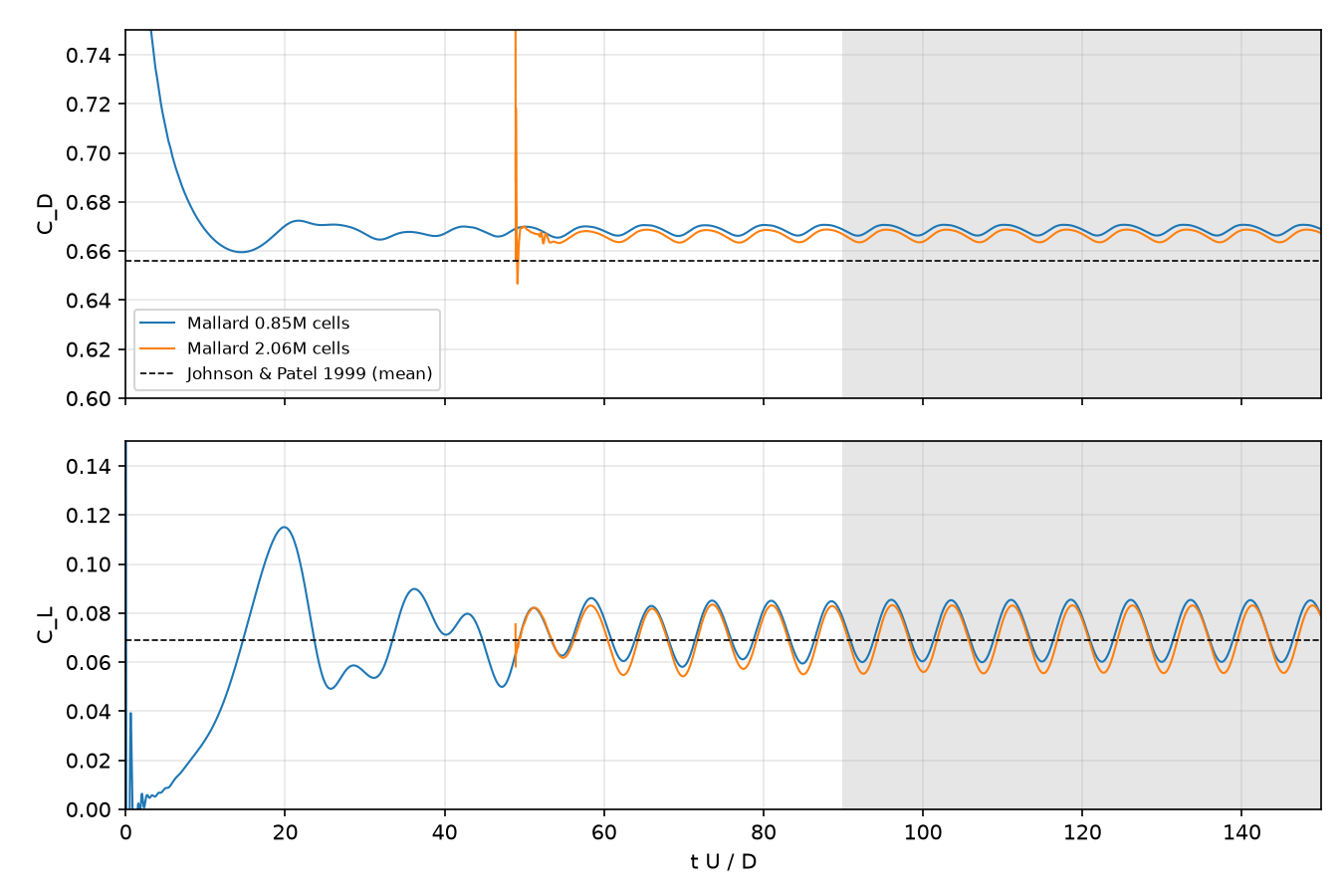
Refining the mesh by 1.4 in every direction changes the Strouhal number by 0.2%, the mean drag by 0.4% and the mean lift by 5%. On the finer mesh the Strouhal number is 1–3% below the references, the mean drag within the spread of the references (0.655 to 0.671), and the mean lift within 7% of them (0.065 to 0.069).

Turbulence

Direct numerical simulations, all in 3D; the large-eddy simulations are in their own section.

Taylor–Green vortex at Re = 1600

256³: e90065d (0.6.0 + 16 commits). 128³: development code shortly after Mallard 0.3.0 (version string 0.3.0; 0.4.0 is the same on hexahedra)

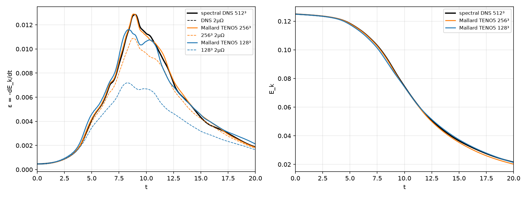
The Taylor–Green vortex is the standard test of a scheme's resolution of transition and decaying turbulence (case C3.5 of the International Workshop on High-Order CFD Methods; Brachet et al. 1983): in the periodic box [0, 2π]³, the velocity u = sin x cos y cos z, v = −cos x sin y cos z, w = 0 rolls up, breaks down into small vortices and decays, at Re = V₀L/ν = 1600, Mach 0.1 and Pr = 0.71. Mallard computes the full periodic box (examples/taylor_green_3d/input_periodic.toml) with fifth-order TENO-E, HLLC and SSPRK3, including the low-Mach correction of the convective flux, to t = 20, at two resolutions:

• 256³ hexahedra (16.8 million cells), CFL 0.4: 65,162 time steps, 0.52 s per step on 14 NVIDIA A100 GPUs over four nodes (about 9.5 hours of stepping).
• 128³ hexahedra (2.1 million cells), CFL 0.8 with the defaults of Mallard 0.3.0: 32,274 time steps, 1 h 18 min on 8 A100 GPUs.

The reference is the workshop's 512³ pseudo-spectral DNS. The resolved dissipation 2μΩ is computed from the enstrophy of the TENO-E reconstruction polynomials' velocity gradients.

256³: Q-criterion isosurfaces colored by vorticity magnitude in the full periodic box, and the dissipation rate traced over the 512³ spectral DNS and the 128³ run.

Dissipation rate −dE_k/dt and its resolved part 2μΩ (left), and mean kinetic energy (right), at 256³ and 128³ against the 512³ spectral DNS.

	512³ DNS	256³	128³
peak of −dEk/dt, at t	0.01286 at 8.97	0.01289 at 8.83 (+0.3%)	0.01161 at 8.39 (−9.7%)
largest |ε − εDNS|, t = 0.5–20, over the DNS peak		3.4%	14.1%
RMS ε error, over the DNS peak		1.2%	4.0%
peak of the resolved 2μΩ	0.01286	0.01087 (−15%)	0.00719 (−44%)
Ek error, t ≤ 12		below 1%	up to 2.6%
Ek at t = 20	0.02157	0.02021 (−6.3%)	0.02134 (−1.1%)

• Shape: at 256³ the dissipation rate follows the DNS through its peak and the shoulder at t ≈ 10–11. At 128³ the peak is 10% low and 0.6 time units early, and the shoulder is lower.
• Resolved and numerical dissipation: the resolved part 2μΩ rises from 56% of the DNS peak at 128³ to 85% at 256³; the rest is numerical, supplied by the scheme in place of the scales the grid cannot represent.
• Late decay: 256³ dissipates slightly more than the DNS (ε within about 5% for t = 12–17), which accumulates to E_k 6% low at t = 20. The 128³ E_k at t = 20 is closer only because its under-dissipation near the peak compensates.

The 128³ run: mean kinetic energy, and the dissipation rate −dE_k/dt and its resolved part 2μΩ, against the 512³ spectral DNS, for which the two coincide.

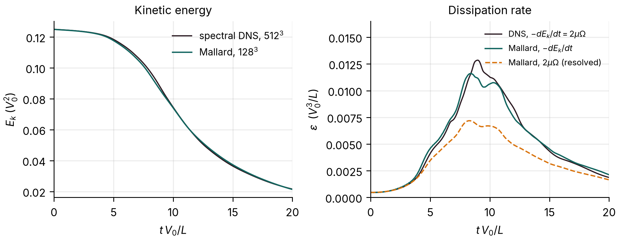
t	5	9	12	20
Ek, Mallard 128³	0.1177	0.0847	0.0550	0.0213
Ek, spectral DNS 512³	0.1184	0.0864	0.0544	0.0216

Decaying compressible isotropic turbulence

Development code between 0.5.0 and 0.6.0: the branch of #170 (version string 0.5.0), merged before 0.6.0

The code-comparison case of Johnsen et al. (2010), computed as a direct numerical simulation with no turbulence model (the isotropic_turbulence example): a random solenoidal velocity field with spectrum E(k) ∼ k⁴ exp(−2 (k/k₀)²), k₀ = 4, in the periodic box [0, 2π]³, with uniform density and pressure, turbulent Mach number M_t,0 = 0.6 and Re_λ,0 = 100, μ ∼ T^3/4 and Pr = 0.7, run to t/τ = 4. The thermodynamic state is out of equilibrium with the velocity, so acoustic waves and entropy modes appear at once, and eddy shocklets form in compressive regions, at local Mach numbers up to 1.9. Fifth-order TENO-E, HLLC and SSPRK3 at CFL 0.4, with the low-Mach correction, on 64³, 128³ and 256³ hexahedra from the same band-limited initial field. Both references filter their solutions to 64³: Johnsen et al. a 256³ solution differentiated with sixth-order differences, Subramaniam et al. (2019) a 512³ DNS with spectral derivatives. Mallard's snapshots are filtered the same two ways. At 256³ (16.8 million cells, 4,307 steps) the run took about an hour on 12 A100 GPUs. The figures are drawn by tools/plot_isotropic_turbulence.py in the Mallard repository.

256³: Q-criterion isosurfaces colored by dilatation (red: compression), dilatation on a plane, and the enstrophy and dilatation variance against Johnsen et al.

Statistics filtered to 64³: kinetic energy, enstrophy, dilatation variance and temperature variance against Johnsen et al. (top, sixth-order differences), and the same with the density variance against Subramaniam et al. (bottom, spectral derivatives).

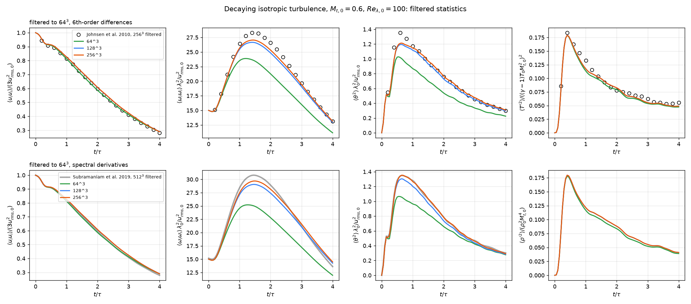
256³, t/τ = 0.2–4, mean / largest difference	kinetic energy	enstrophy	dilatation variance	temperature variance
vs Johnsen et al., 256³ filtered to 64³	+2.1% / +3.2%	−2.4% / −4.8%	−0.5% / −14% (t/τ = 0.4)	−4.9% / −12%
vs Subramaniam et al., 512³ filtered to 64³	+2.3% / +4.0%	−0.3% / +6.5%	−0.6% / −4.9%

Shell spectra of velocity, vorticity, dilatation and density at t/τ = 2 and 4 against Subramaniam et al.; each reference spectrum is scaled by one fitted factor, since its normalization is not stated.

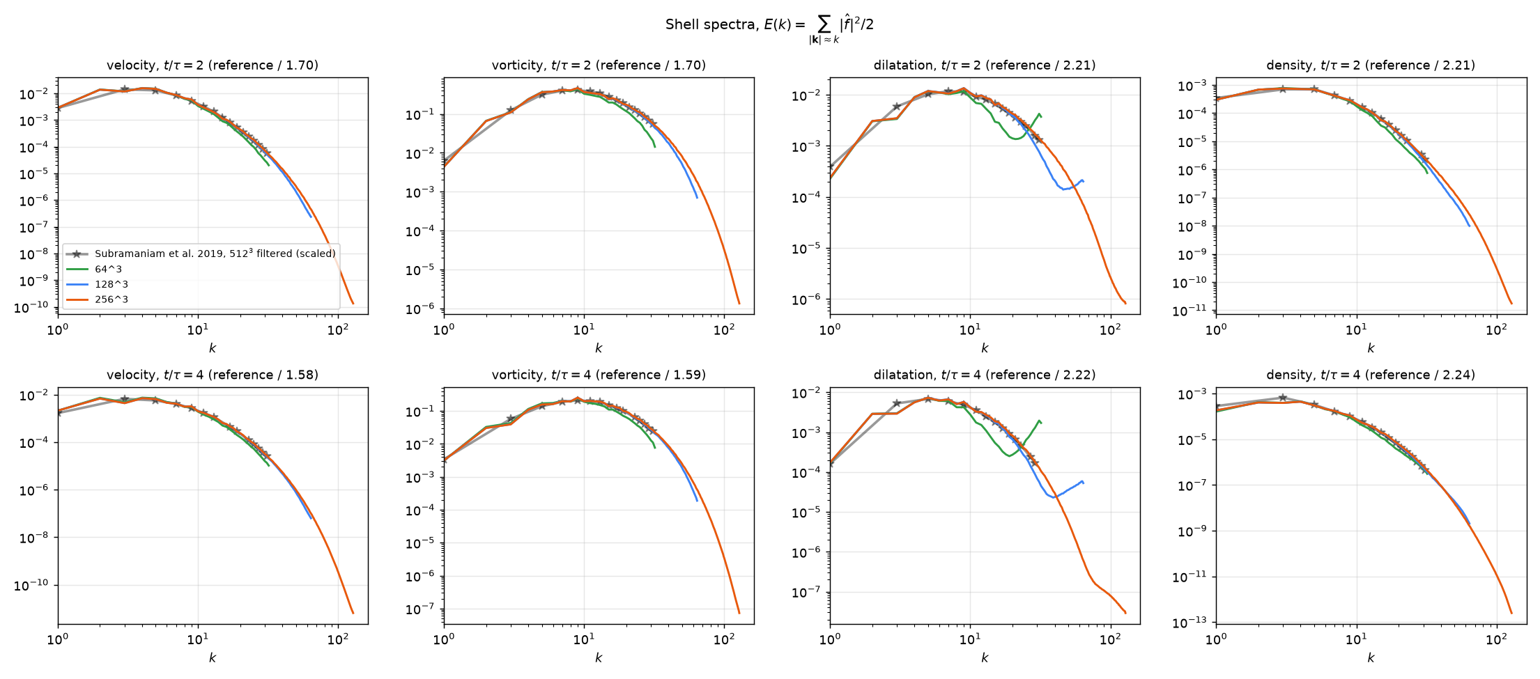
• Resolution: k_maxη stays above 2.71 at 256³ (1.36 at 128³, 0.71 at 64³). At 256³ the velocity spectrum falls 8 decades by the grid cutoff, and TENO flags at most 3.4% of the cells (64³: 76%), so the scheme mostly runs on its linear fifth-order stencils.
• Grid convergence, 128³ against 256³, unfiltered: kinetic energy, temperature and density variances within 0.3%; enstrophy 2.5% mean; dilatation variance 6% mean and 13% at its peak, carried by the steepest shocklets, only a few cells thick. Filtered to 64³, the two grids differ by under 2% in enstrophy and 5% in dilatation. 64³ misses 18% of the enstrophy.
• Remaining offsets (kinetic energy +2%, temperature variance −5%) are larger than the grid error and about as large as the spread between random initial fields: three seeds at 64³ differ by ±1% in kinetic energy and ±3% in temperature variance at t/τ = 4. The references' realizations are not published.
• Spectra at t/τ = 2 and 4 have the shape of Subramaniam et al.'s within 0.02–0.09 decades RMS.
• Low-Mach correction: most faces are subsonic, so it is active; turning it off lowers the filtered enstrophy by 10% at 64³ and 2% at 128³.

Turbulent channel flow, Re_τ = 180

Example run: c7384ae (0.6.0 + 33 commits). The variants with the Riemann solver at every face: 9de2a0e (between 0.5.0 and 0.6.0)

Direct numerical simulation of turbulent channel flow at Re_τ = 180, against the spectral DNS of Moser, Kim & Mansour (1999, MKM), the channel_retau180 example, with the kinetic-energy-preserving hybrid convective flux (#205, #216). It uses MKM's box, 4πh × 2h × 4/3πh, periodic in x and z, between isothermal walls at bulk Mach 0.2. The mass flow is held at Re_b = 5600, so Re_τ is an outcome of the run. The mesh is 192 × 96 × 128 hexahedra (2.36 million), tanh-stretched in y: Δx⁺ = 11.8, Δz⁺ = 5.9, Δy⁺ = 0.88 at the wall. Navier–Stokes with no turbulence model. MUSCL states with the hybrid flux, which is the central KEEP flux everywhere except where the compression sensor calls the Riemann solver. Statistics are averaged over t = 120–320 h/U_b (12.9 h/u_τ), with both halves of the channel folded. The run took 489,000 steps, 2.3 hours on two A100 GPUs.

Near-wall vortices (Q⁺ = 0.01, colored by streamwise velocity) over the low- and high-speed streaks at y⁺ = 11.

Mean velocity, RMS velocity fluctuations and Reynolds shear stress in wall units against MKM, and Re_τ(t) from the wall shear with the averaging window.

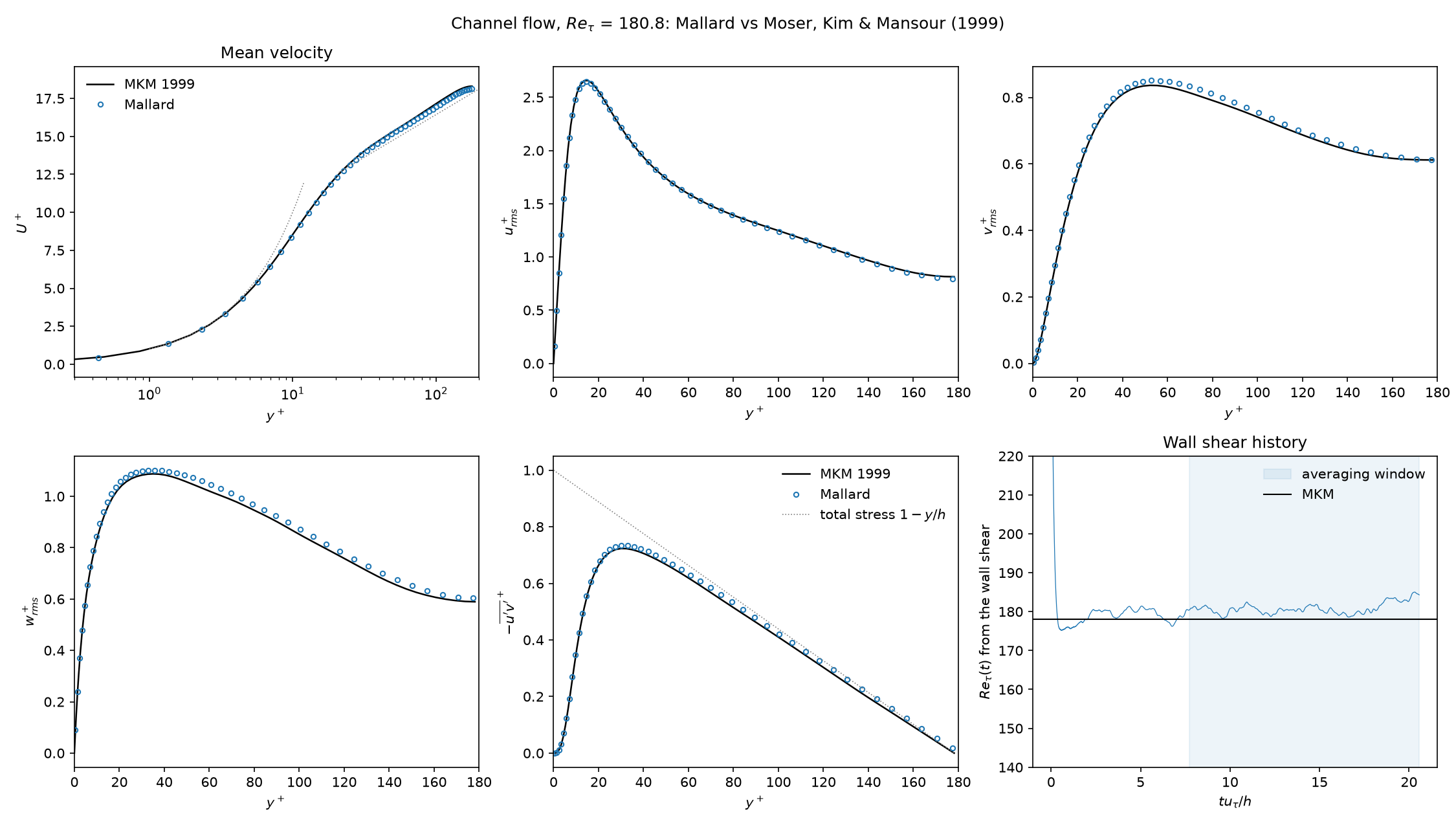
	Mallard	MKM	difference
Reτ	180.8	178.1	+1.5%
Cf = 2τw / ρUb²	0.00830	0.00814	+2.0%
peak urms+	2.645	2.658	−0.5%
peak vrms+	0.851	0.836	+1.8%
peak wrms+	1.102	1.087	+1.4%
peak −u′v′+	0.734	0.723	+1.5%

The kinetic-energy budget of [integrals] attributes 0.9% of the dissipation to the scheme and the rest to molecular viscosity. A second run, continued from a developed state and averaged over t = 365–560, reproduces these values to 0.5%. The mean momentum balance closes to 0.6% of τ_w.

The upwind dissipation of a Riemann solver at every face sets the friction. Each variant below starts from the same developed state and averages over 12 h/u_τ (#209):

Convective flux and mesh	Reτ	Cf vs MKM	peak urms+
HLLC, low-Mach correction (cutoff 0.1)	172.9	−6.8%	2.894
Roe	171.9	−7.9%	2.913
HLLC, low-Mach cutoff 0.01	173.9	−5.8%	2.872
HLLC, low-Mach correction off	157.1	−23.0%	3.343
HLLC with TENO3 instead of MUSCL	169.3	−10.6%	2.926
HLLC, 384 × 96 × 128 (Δx+ 6)	174.1	−5.5%	2.822
HLLC, 192 × 96 × 256 (Δz+ 3)	176.8	−2.6%	2.803
HLLC, 384 × 96 × 256	178.4	−0.8%	2.716
hybrid (KEEP central), continuation window	181.0	+2.1%	2.648

On the example's mesh HLLC removes about 7% of the kinetic-energy dissipation, and the wall shear comes out 7% low. Without the low-Mach correction its dissipation is about five times larger in the core, and C_f is 23% low. HLLC reaches MKM, with v_rms, w_rms and −u′v′ within 2%, only with both Δx and Δz halved, at about five times the GPU time. Halving the time step changes nothing to 1%.

Synthetic turbulent inflow

f7d6571 (0.6.0 + 77 commits, the branch of #221)

A spatially developing channel at Re_τ = 180 fed by synthetic turbulence, the channel_inflow_retau180 example (#221); setting it up (and the design notes).

• Inflow: the nscbc_inlet takes its mean velocity and Reynolds stresses from the statistics of the periodic channel. The digital filter of Klein, Sadiki & Janicka (2003) adds turbulence with those stresses, with integral lengths of 0.5h (streamwise velocity) and 0.1–0.2h otherwise.
• Domain: the periodic example's mesh twice as long, 8πh (384 × 96 × 128), with a sponge before the outlet beyond x = 20h.
• Statistics: averaged over t = 40–110 and over z, compared with the periodic channel at each x.
• Cost: 337,000 steps, 2.5 hours on four A100 GPUs. DNS, no turbulence model.

Wall shear, Re_τ and the peaks of the Reynolds stresses along the channel, over their values in the periodic channel; the band is ±5%.

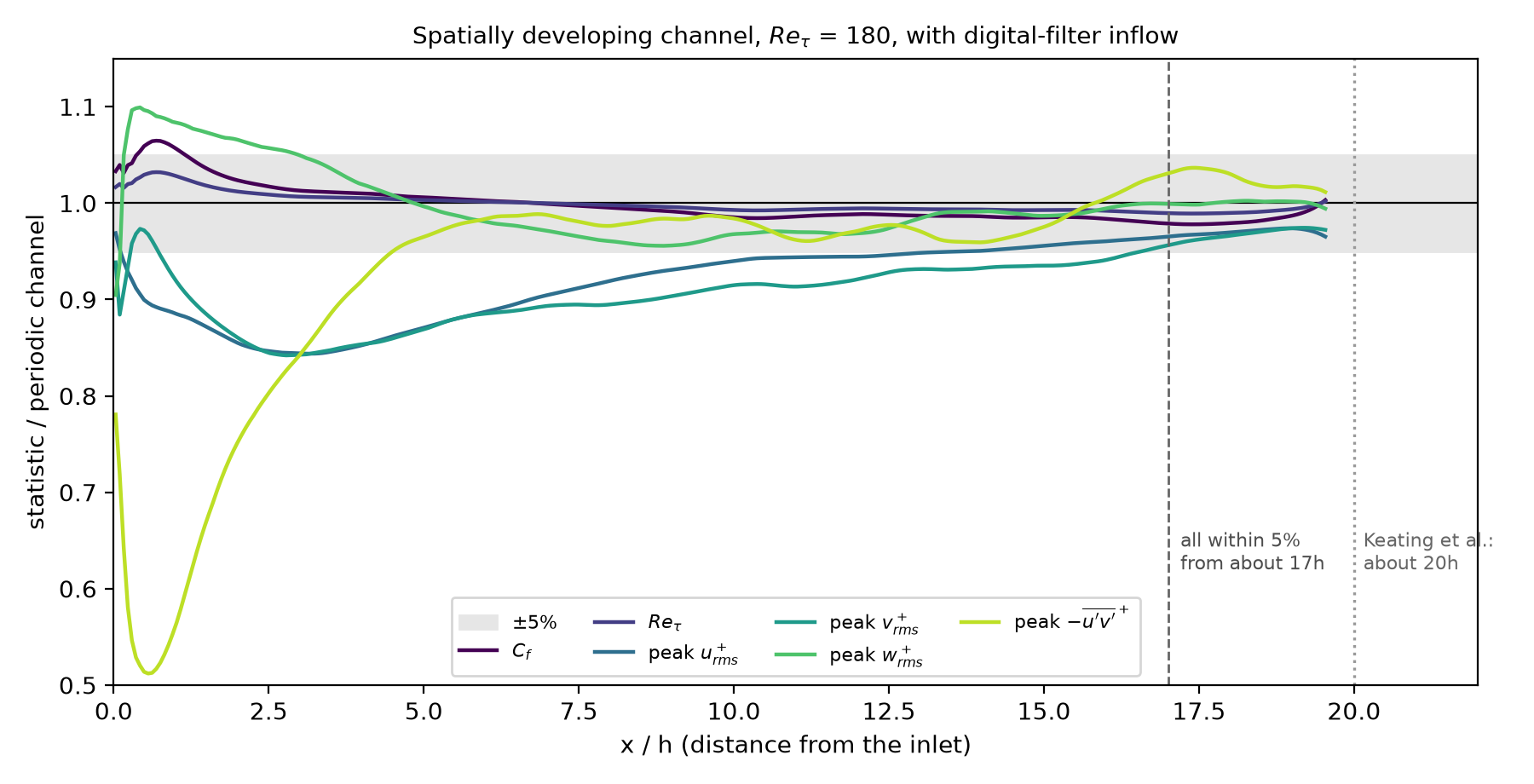
Statistic	within 5% of the periodic channel from
Reτ	the inlet
Cf	1.1h
peak wrms+	2.9h
peak −u′v′+	4.6h (57% of it at the inlet)
peak urms+	13.7h
peak vrms+	16.6h

Every statistic is within 5% from about 17h; Keating et al. (2004) report about 20h for synthetic inflow into a channel. The shear stress recovers quickly because the full Reynolds-stress tensor and the precursor's mean profile are imposed. The normal stresses take longest: u_rms and v_rms first dip to about 85% at x = 2–4h, as the inflow sheds its non-turbulent, dilatational part.

Reacting flow

Mallard 0.4.0 added thermally perfect gas mixtures and finite-rate chemistry: mechanisms in Cantera's YAML format, mixtures carried by the flow solver (MUSCL or TENO-E, optionally with double flux), kinetics with an analytical Jacobian integrated by a Rosenbrock method (RODAS), Strang splitting between chemistry and flow, and mixture-averaged, unity- or constant-Lewis-number transport; 0.5.0 runs the chemistry efficiently on GPUs (performance). It is set up with gas = "mixture" in [physics] and the [chemistry] table. The thermochemistry guide explains how to set them up (and the design notes the choices behind them); the cases below are its V1, V2 and V6 to V8, and two 2D demonstrations, a cellular detonation and a lean hydrogen flame. They use the H₂/O₂ submechanism of GRI-Mech 3.0 with Ar and N₂ (mechanisms/h2o2.yaml: 10 species, 29 reactions) or the full GRI-Mech 3.0 (53 species, 325 reactions), with the default chemistry tolerances (relative 10⁻⁶, absolute 10⁻¹⁰). The shock and detonation cases are inviscid; the flames include molecular transport.

Ignition

Mallard 0.4.0

MallardReactor, a tool built with Mallard, integrates an adiabatic constant-volume reactor with the solver's chemistry kernels (the h2_ignition example). It ran H₂/air and CH₄/air at T₀ = 1000 to 1500 K, equivalence ratios φ = 0.5, 1 and 2 and 1 atm, 36 mixtures, against Cantera's IdealGasReactor with tolerances of 10⁻¹², both sampled at the same 1500 times (1000 per ignition delay); the ignition delay is the time of the largest dT/dt.

Left: temperature of stoichiometric H₂/air from 1200 K and 1 atm. Right: ignition delays of the 36 mixtures.

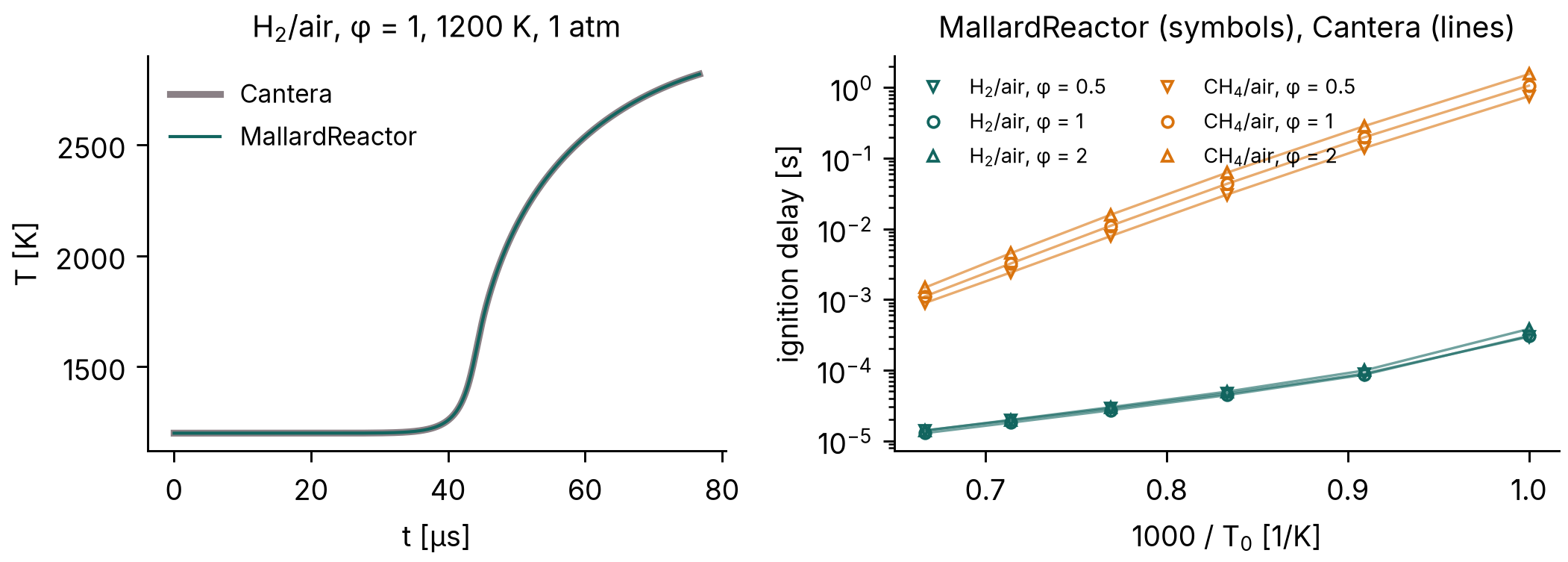
The ignition delays agree with Cantera's within 2.7 × 10⁻⁶ (relative) for H₂/air and 1.8 × 10⁻⁴ for CH₄/air, whose largest differences are at 1000 K, where ignition takes 0.9 to 1.6 s; from 1100 K up both are within 10⁻⁷. Run on to equilibrium (200 ignition delays for H₂/air, 2 s for CH₄/air), every reactor ends within 2 × 10⁻⁶ K of Cantera's constant-volume equilibrium temperature. Mallard's test suite repeats these comparisons, against stored Cantera data, on every change.

Reactive shock tube

Mallard 0.4.0

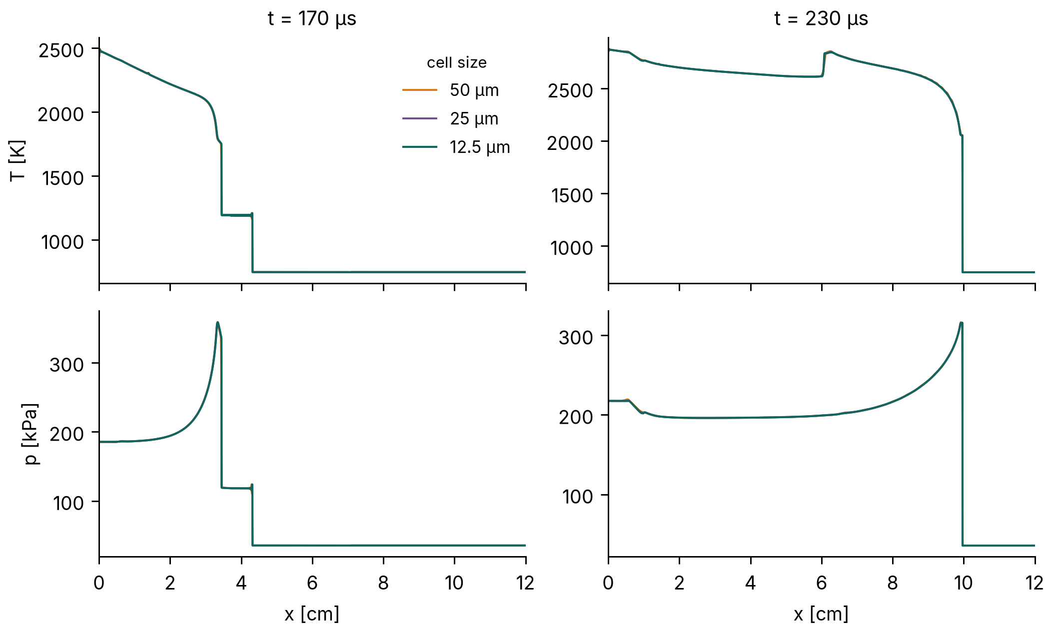
The reactive shock tube of Fedkiw, Merriman & Osher (1997), studied in detail by Martínez Ferrer et al. (2014): in H₂:O₂:Ar = 2:1:7, a shock running into the closed end of a 12 cm tube reflects, the gas behind the reflected shock ignites, and the reaction front turns into a detonation that overtakes the reflected shock. The reactive_shock_tube example starts from the published states (p, T, u) = (7173 Pa, 378 K, 0) for x < 6 cm and (35,594 Pa, 748 K, −487 m/s) beyond, on 2400, 4800 and 9600 cells (50, 25 and 12.5 µm), with MUSCL, HLLC and SSPRK3 at CFL 0.5.

Temperature and pressure at 170 µs, as the detonation forms behind the reflected shock, and at 230 µs, after it has overtaken it.

Cell size	Front at 170 µs	Front at 230 µs	Peak T at 230 µs	Peak p at 230 µs
50 µm	33.23 mm	99.63 mm	2875.2 K	316.6 kPa
25 µm	33.29 mm	99.66 mm	2876.1 K	316.0 kPa
12.5 µm	33.33 mm	99.66 mm	2876.6 K	315.7 kPa

The front is the last cell above 1800 K. At 230 µs the three meshes put the detonation within one 50 µm cell of each other (99.625, 99.662 and 99.656 mm), and the peak temperature and pressure behind it change by less than 0.05% and 0.1% from 25 to 12.5 µm; at 170 µs the reaction front, still behind the reflected shock (near 4.3 cm), moves by 0.04 mm between the two finest meshes.

CJ detonation

Mallard 0.4.0

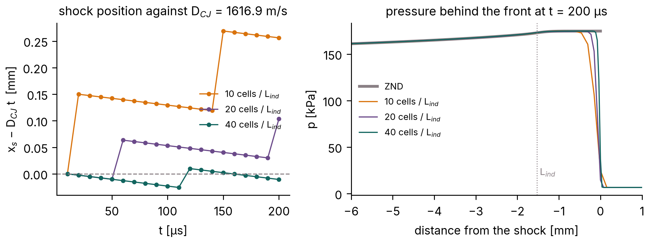
A planar Chapman–Jouguet detonation in 2H₂-O₂-7Ar at 6.67 kPa and 298 K, the detonation_1d example. With this mechanism the recombination zone behind the front is about 0.8 m long, so a detonation started by a driver gas runs below the CJ speed over any practical tube (9% below over 0.6 m); the run therefore starts from the steady ZND structure, computed with Cantera by tools/detonation_reference.py (the formulation of Shepherd's Shock and Detonation Toolbox) and placed on the mesh by tools/znd_restart.py, and must keep it: the CJ speed D_CJ = 1616.9 m/s, the induction length (from the shock to the peak heat release) 1.525 mm, and the von Neumann pressure spike, 174.7 kPa. A 0.6 m tube with the shock at 0.25 m, run for 200 µs (about 0.32 m of travel) on 10, 20 and 40 cells per induction length; MUSCL, HLLC, SSPRK3 at CFL 0.5. The front speed is a line fit to the shock position (the last cell above twice the initial pressure) over the second half of the run, and the induction length the mean over the same outputs.

Left: front speed between outputs 10 µs apart. Right: pressure behind the front at 200 µs against the ZND profile; the dotted line is the ZND induction length.

Cells per induction length	Front speed	vs DCJ	Induction length	vs ZND	Peak pressure
10 (152.5 µm)	1618.8 m/s	+0.11%	1.456 mm	−4.5%	174.8 kPa
20 (76.3 µm)	1617.0 m/s	+0.01%	1.497 mm	−1.8%	175.2 kPa
40 (38.1 µm)	1617.0 m/s	0.00%	1.567 mm	+2.7%	174.7 kPa
ZND	1616.9 m/s		1.525 mm		174.7 kPa (von Neumann)

The front keeps the CJ speed to 0.01% from 20 cells per induction length: the shock stays within two cells of the position of a wave moving at D_CJ (left of the figure; the shock position moves in whole cells). The induction length is within 5% of the ZND value at all three resolutions, a difference of at most one cell at 40 (2.5%), and the peak pressure, the largest over the second half of the run, matches the von Neumann pressure, the pressure right behind a non-reacting shock at D_CJ.

Laminar flame speed

Mallard 0.4.0

Freely propagating premixed H₂/air flames at 300 K and 1 atm, φ = 0.6 to 1.4, with mixture-averaged and unity-Lewis-number transport, against Cantera's FreeFlame with the same mechanism and transport model (the premixed_flame example). Each run is a strip in the flame's frame, started from Cantera's flame, from 6 thermal thicknesses δ_T upstream of the flame to 9 downstream, with 20 cells per δ_T; the fresh mixture enters at Cantera's flame speed, and the flame speed is the consumption speed of the deficient reactant, averaged over the last third of two flame times δ_T/S_L. Navier–Stokes, MUSCL, HLLC, SSPRK3 at CFL 0.4.

Left: flame speeds with both transport models. Right: temperature through the stoichiometric flame with mixture-averaged transport.

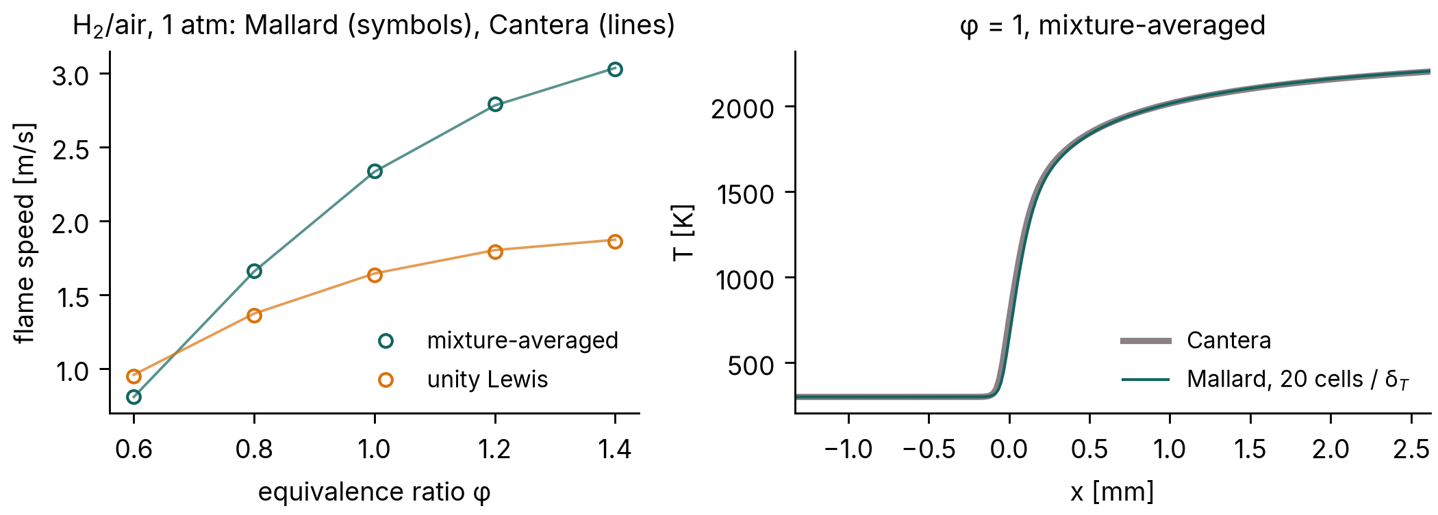
φ	0.6	0.8	1.0	1.2	1.4
Cantera, mixture-averaged [m/s]	0.8075	1.6567	2.3317	2.7806	3.0341
Mallard	+0.38%	+0.31%	+0.24%	+0.32%	−0.20%
Cantera, unity Lewis [m/s]	0.9575	1.3716	1.6431	1.8013	1.8713
Mallard	−0.81%	−0.72%	−0.68%	−0.65%	−0.56%

All ten flame speeds are within 0.81% of Cantera's (the lean mixture-averaged run stopped after 1.35 of its two flame times). For CH₄/air at φ = 1 with GRI-Mech 3.0, the design note reports −0.93% (mixture-averaged) and −0.04% (unity Lewis).

Laminar flame speed, CH₄/air

040fb35 (0.6.0 + 114 commits), merged in #241; first released in Mallard 0.8.0

Freely propagating CH₄/air flames at 300 K and 1 atm with GRI-Mech 3.0 (53 species, 325 reactions), φ = 0.6 to 1.4, with mixture-averaged and unity-Lewis-number transport, against Cantera's FreeFlame with the same mechanism and transport (#241). Each flame starts from Cantera's and runs five flame times at CFL 1, at 10, 20 and 40 cells per thermal thickness, on A100 GPUs; the consumption speed is taken over the last flame time.

Left: flame speeds at 20 cells per thermal thickness against Cantera. Right: consumption-speed error at 10, 20 and 40 cells.

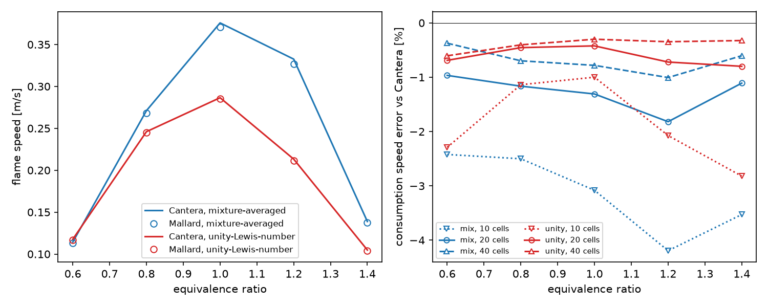
φ	0.6	0.8	1.0	1.2	1.4
Cantera, mixture-averaged [m/s]	0.1144	0.2711	0.3758	0.3325	0.1388
Mallard, 10 / 20 / 40 cells	−2.42 / −0.97 / −0.37%	−2.50 / −1.17 / −0.70%	−3.08 / −1.31 / −0.78%	−4.19 / −1.82 / −1.01%	−3.53 / −1.11 / −0.60%
Cantera, unity Lewis [m/s]	0.1177	0.2460	0.2865	0.2132	0.1048
Mallard, 10 / 20 / 40 cells	−2.29 / −0.69 / −0.61%	−1.14 / −0.45 / −0.40%	−1.00 / −0.42 / −0.30%	−2.07 / −0.72 / −0.35%	−2.82 / −0.80 / −0.32%

At 20 cells per thermal thickness every flame speed is within 2% of Cantera's: mixture-averaged 1.0–1.8% slow, unity Lewis 0.4–0.8% slow. At 40 cells the mixture-averaged errors roughly halve. Some 40-cell runs ran 2.2–4.1 rather than five flame times and are still settling slowly downward. Halving the CFL number changes the flame speeds by at most 0.05%.

Thermal diffusion (Soret effect)

caa9b4a with local changes (0.6.0 + 125 commits), merged in #243; first released in Mallard 0.8.0

physics.soret = true adds thermal diffusion to the species fluxes with mixture-averaged transport, using Cantera's mixture-averaged thermal-diffusion coefficients (#243). The test case is freely propagating H₂/air flames at 300 K and 1 atm against Cantera's FreeFlame with and without thermal diffusion: the setup of the H₂ flame speeds, with 20 cells per thermal thickness, CFL 0.2 and two flame times.

φ	0.4	0.5	0.6	1.0
consumption speed vs Cantera, without Soret	+0.40%	+0.19%	+0.28%	+0.21%
consumption speed vs Cantera, with Soret	−0.58%	−0.07%	+0.34%	+0.41%
change from thermal diffusion, Cantera / Mallard	−3.10 / −4.05%	−6.98 / −7.23%	−9.04 / −8.98%	−8.44 / −8.26%

Mallard reproduces Cantera's reduction of the flame speed by thermal diffusion to within 0.3 percentage points from φ = 0.5 to 1.0, and to 1 point at φ = 0.4. The coefficients themselves match Cantera's to 6 × 10⁻¹³ of the largest. Runs without the option are byte-identical to those before the change.

Optically thin radiation

2d7dde7 (merge of #226); first released in Mallard 0.8.0

[radiation] adds an optically thin radiative loss, q = 4σ Σ p_i a_P,i(T) (T⁴ − T_ambient⁴), with the TNF workshop's Planck-mean coefficients for H₂O, CO₂, CO and CH₄ (#226). The loss matches Cantera 3.2's radiative_heat_loss to 10⁻⁹. The flames below are freely propagating CH₄/air flames against Cantera's FreeFlame with the same radiation model (H₂O and CO₂), at 12 cells per flame thickness.

Mixture	Srad/Sad, Cantera	Mallard
CH4/air, φ = 0.6, GRI-3.0	0.9738	0.9735
CH4/air, φ = 0.5, GRI-3.0	0.811	0.808
CH4/air, φ = 0.44, two-step (2S-CH4-BFER)	0.8509	0.8507

Radiative flammability limit (two-step mechanism): Cantera finds a radiating flame at φ = 0.41 and none at 0.405. Mallard's flame at φ = 0.41 burns at 2.152 cm/s (Cantera 2.181). At φ = 0.40, started from the adiabatic profile, it slows from 2.0 to 0.2 cm/s within 17 flame times and goes out.

Flame–vortex quenching

2d7dde7 (merge of #226); first released in Mallard 0.8.0

The flame–vortex interactions on the spectral diagram of Poinsot, Veynante & Candel (1991), with the heat losses their quenching needs, in the flame_vortex_quenching example (#226).

• Flame: lean CH₄/air at φ = 0.42, 3% above its radiative limit, with the two-step 2S-CH4-BFER mechanism (Franzelli et al. 2012) and the TNF radiation model. S_L = 2.69 cm/s and δ_L = 3.0 mm.
• Vortex pairs: sizes r of 1 to 8 δ_L and velocities u′ of 3 to 100 S_L.
• Resolution: 12 cells per δ_L, or 24 for r = 1.
• Classification: the analysis puts each run in one of Poinsot et al.'s four classes:
  • no effect: the heat release changes by less than 5%
  • wrinkled
  • pocket: fresh gas cut off and burnt out
  • quenched: the front goes out and fresh gas reaches the outlet

The twelve runs at φ = 0.42: temperature, with heat release in white and the vortices' vorticity in blue and pink, their places on the spectral diagram, and their heat release over time.

r/δL \ u′/SL	3	10	30	40	100
1			no effect		wrinkled
2		no effect	wrinkled		quenched
4	no effect	wrinkled	quenched		quenched
8		pocket		quenched	quenched

Left: outcomes on the spectral diagram, with the range of Poinsot et al.'s runs and their quenching example. Middle: heat release over the planar flame's. Right: the weakest burning along the front.

The pair r = 4 δ_L, u′ = 30 S_L against the radiating flame at φ = 0.42 (quenched), at φ = 0.44 (weaker losses: the pocket burns out) and without radiation at φ = 0.42 (burns out), with r = 8 δ_L, u′ = 40 S_L for comparison.

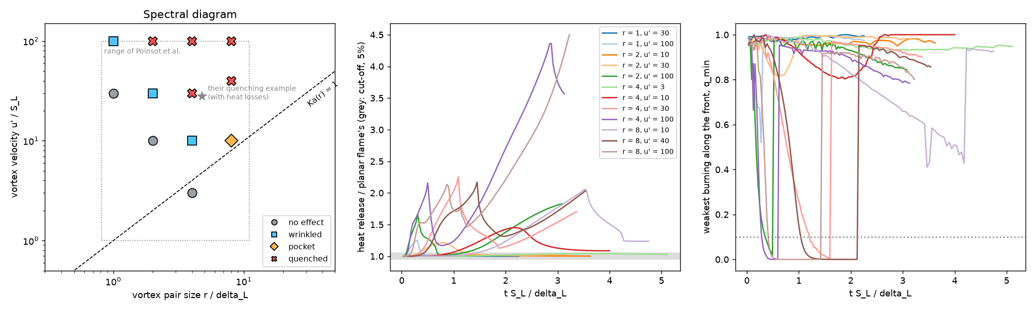
• How quenching happens: each pair that quenches cuts off a pocket of fresh gas and pushes it into burnt gas that radiation has cooled by 100–300 K. The pocket's downstream side goes out, and 30–100% of the inlet CH₄ reaches the outlet unburnt. This is Poinsot et al.'s quenching example (r/l_F = 4.8, u′/S_L = 28).
• Radiation decides it: the same pair (r = 4, u′ = 30) leaves a pocket that burns out at φ = 0.44 with radiation, and at φ = 0.42 without radiation.
• Boundary: quenching sets in at Ka(r) between 1.25 and 5 for r = 8, 2.5–7.5 for r = 4 and 15–50 for r = 2, and never up to Ka = 100 for r = 1. The boundary climbs steeply toward small pairs and approaches Ka = O(1) for large ones, the shape of Poinsot et al.'s curve. Their 5% cut-off for small or slow pairs is also reproduced.
• Resolution check: at 24 cells per δ_L, r = 4, u′ = 30 also quenches.
• What does not match:
  • Poinsot et al.'s loss was linear in the temperature and applied to all the gas, with one-step chemistry and a Lewis number of 1.2. Here the loss is radiation, the chemistry has two steps, and CH₄'s Lewis number is about 1. Only the shape and the order of magnitude of the boundary compare, since its position moves with the loss level.
  • Quenched pockets reach the outlet before they are gone.

SIMPLER splitting

beb3c3f with local changes, and 3500760 (0.6.0 + 85 and 87 commits), merged in #235; first released in Mallard 0.8.0

[chemistry] coupling = "simpler" balances the chemistry and the flow with the SIMPLER splitting of Wu, Ma & Ihme (2019) instead of Strang's (#235). The reaction substep sees the transport rate at the start of the step as a constant forcing, so a steady state of the coupled equations is a steady state of the scheme. It stays second order, and Strang remains the default. The checks use H₂/O₂ chemistry with MUSCL, HLLC and SSPRK3.

Case	Strang	SIMPLER
CJ detonation, induction length vs ZND, 10 cells per induction length, CFL 0.35 / 0.5 / 0.7 / 1.0 / 1.2	−4.5 / −5.5 / −8.2 / −25.5 / −36.4%	−7.3 / −7.3 / 0.0 / −0.9 / −5.5%
the same, 20 cells per induction length, CFL 0.35 / 0.7 / 1.0	−1.4 / – / −11.4%	−0.9 / +2.3 / +3.2%
detonation speed, D/DCJ − 1	within 0.16%	within 0.16%
detonation cost (8 CPU threads, 3934 cells)	222 s at CFL 0.35	60 s at CFL 1.0
stirred reactor (H2/air from 300 K), extinction residence time at dt = 0.1 / 0.3 / 1 τ (exact 40–50 µs)	50 µs / 100 µs / > 1 ms	40–50 µs at every dt
stirred reactor, τ = 100 µs, dt = 0.1 τ: temperature	2695.8 K (+24 K)	2671.9 K (exact)
H2/air flame speeds vs Cantera, φ = 0.6 / 1.0 / 1.4	+0.60 to −0.21%	+0.53 to −0.20%

Detonations can therefore run at CFL 1.0 instead of 0.35, 3.7 times cheaper, with the mean induction length within 5% and the detonation speed unchanged. The price is a front position that oscillates more from output to output (5.5% against 0.6% RMS at CFL 1.0 and 10 cells). For steady premixed flames, where Strang's splitting error is already below 0.1%, SIMPLER is only 9–15% cheaper.

Cellular detonation

Development code just before the 0.4.0 release (version string 0.3.0, run 3 October 2026, the branch of #130; commit not recorded), released in 0.5.0

The detonation of the CJ detonation section in two dimensions, the detonation_2d example: a 6 cm wide channel with slip walls, 0.15 mm cells (10 per induction length, as in Oran et al. 1998), 1.2 million cells, 18,900 time steps in 39 minutes on two A100 GPUs, 71% of it in the chemistry. The run starts from the ZND solution with six seeded pockets of fresh gas behind the front: a planar ZND front, with or without one such pocket, stays planar at 5 to 20 cells per induction length, so the cells here grow from the seeds and not from the front's own instability. The [[write_data]] variable P_MAX, the largest pressure each cell has seen, gives the numerical soot foil.

Pressure and the numerical soot foil near the front, and the whole foil below.

The front runs at 1617.0 m/s, the CJ speed to 0.01%. The seeds give eight strong triple points at x = 140 to 180 mm, cells about 15 mm wide, which coarsen to three or four (30 to 40 mm) by x ≈ 260 mm; after 33 cm of travel the cells are not yet regular. Published numerical cell widths for this mixture are about 3 cm (Oran et al. 1998; Deiterding 2011).

Cellular detonation in 3D

Development code between 0.5.0 and 0.6.0: 3bec90f with the tools of #183

The detonation of the previous section in a 3 cm square duct, the configuration of Deiterding's (2011) and Tsuboi et al.'s (2002) 3D runs, in the detonation_3d example. The resolution is that of the 2D case, 0.15 mm hexahedra (10 per induction length), 200 × 200 across the duct. A 7.2 cm window follows the front: 480 × 200 × 200 = 19.2 million cells. Every 6 µs the run drops the burnt gas more than 5 cm behind the front, appends fresh gas ahead, and keeps the peak pressure of the dropped wall cells for the soot foils. The run starts from a 2D cellular detonation turned into in-phase transverse waves in y and z. MUSCL with HLL: HLLC grows grid-scale odd–even noise on the planar 3D front within 15 µs. The run took 12,180 steps, 4.6 hours on four A100 GPUs.

The leading shock colored by the pressure behind it, the soot foils on the two far walls, and the foils of all four walls over 17 cm of travel.

Over t = 96–204 µs (17 cm of travel), the front runs at 1620.6 m/s over the second half, D_CJ to 0.2%. Its transverse waves stay as two orthogonal families of lines parallel to the walls, crossing in phase. This is the rectangular mode of Deiterding's and Tsuboi et al.'s runs. The peak pressure behind the shock stays at 200–215 kPa (von Neumann: 175 kPa) to the end, while in the 2D precursor it decays. On every wall the foil shows diagonal triple-point tracks crossing every 6.4 cm of travel (6.5 cm in the 2D precursor). It also shows dark bands across the whole wall, every 4–8.6 cm and alternating between opposite walls, where a wave family hits the wall face-on (the slapping waves of Williams, Bauwens & Oran 1996). The start is symmetric under exchanging y and z, and so is the solution: the foils of opposite wall pairs are identical.

Lean hydrogen flame

Development code just before the 0.4.0 release (version string 0.3.0, run 3 October 2026, the branch of #131; commit not recorded), released in 0.5.0

A lean H₂/air flame, φ = 0.4, 700 K, 1 atm, in a periodic channel 7.8 mm wide and 12.2 mm long on 36 µm cells (72,576), started from the same wrinkled planar flame with mixture-averaged transport and with unity Lewis numbers (the flame_2d example; 82 and 67 minutes on one A100). On the same mesh, the planar flame runs at 3.3446 m/s (mixture-averaged) and 3.1093 m/s (unity Lewis), against Cantera's 3.346 and 3.129 m/s (−0.04% and −0.6%).

Temperature over the adiabatic flame temperature with mixture-averaged transport (left) and unity Lewis numbers (right), and the consumption speeds over the planar flame's.

With unity Lewis numbers the burnt gas stays within 0.996 to 1.000 of the adiabatic flame temperature T_ad, and the wrinkle grows only by the Darrieus–Landau instability: the consumption speed peaks at 1.08 S_L at 2.4 ms. With mixture-averaged transport, the differential diffusion of hydrogen makes the burnt gas behind the bulges superadiabatic, from 0.958 to 1.017 T_ad, and the consumption speed peaks at 1.14 S_L at 1.1 ms.

Stratified autoignition

Development code between 0.5.0 and 0.6.0: bdca83d with the tools of #174

Autoignition of a thermally stratified lean H₂/air mixture at constant volume, the configuration of the DNS of Chen et al. (2006), Hawkes et al. (2006) and Sankaran et al. (2005), in the autoignition_2d example.

• Mixture: φ = 0.1, a mean 1070 K and 41 atm, in a 4.1 mm periodic square.
• Initial fields: random temperature fluctuations T′ of 3.75, 7.5, 15 and 30 K, and decaying turbulence (u′ = 0.5 m/s). Both follow Passot–Pouquet spectra with most energetic lengths of 1.25 mm, from one seed.
• Mesh and models: 400 × 400 cells of 10.25 µm, 11–15 per deflagration thickness. H₂/O₂ chemistry and mixture-averaged transport.
• Reference delay: τ₀ = 3.650 ms, the homogeneous ignition delay, from both Cantera and MallardReactor.
• Cost: 1.4–2.0 million steps per run, 4.7–5.5 hours on four A100 GPUs.

Temperature (top) and heat release rate (bottom) of the four runs, and their mean heat release rate against the multizone model and the homogeneous reactor.

Mean heat release rate over the homogeneous reactor's peak: DNS (solid), multizone model of each initial field without transport (dashed), homogeneous reactor (dotted).

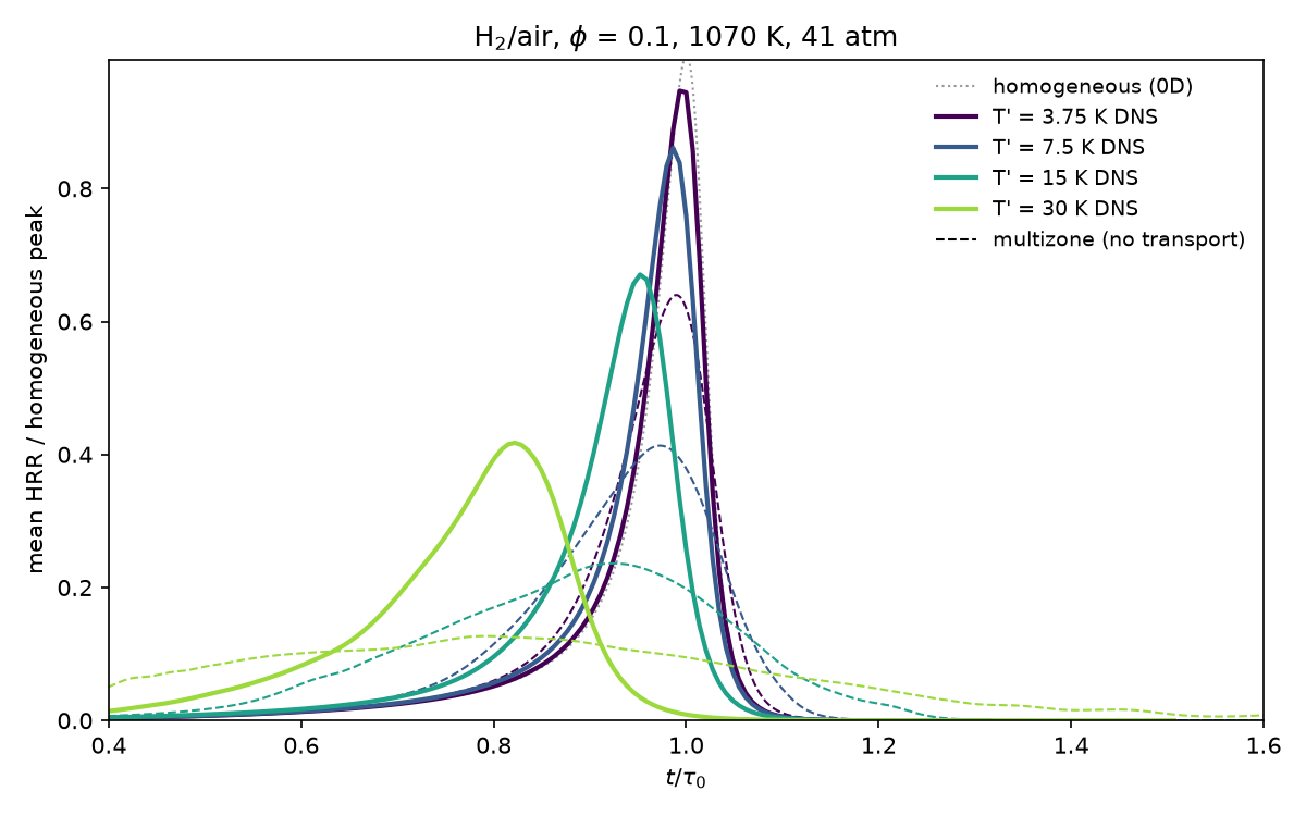
T′ [K]	peak time / τ0	FWHM / τ0	peak / homogeneous	deflagrative share	median front speed
3.75	0.993 (0.990)	0.062 (0.110)	0.95 (0.64)	0.0%	16.7 SL
7.5	0.986 (0.973)	0.069 (0.187)	0.86 (0.41)	0.2%	9.1 SL
15	0.952 (0.924)	0.089 (0.354)	0.67 (0.24)	2.9%	5.1 SL
30	0.822 (0.791)	0.164 (0.697)	0.42 (0.13)	25%	2.4 SL

Columns 2–4 describe the mean heat release rate; the multizone model is in brackets. The deflagrative share is the heat released where the H₂O isolines move slower than 1.5 S_L. The median front speed is the heat-release-weighted median of the displacement speed |S_d^*| over the deflagration speed S_L(T_u, p) of the local fresh gas.

Peak time, burn duration and deflagrative share against T′: DNS, multizone model, and Sankaran et al.'s β criterion applied to the initial field and at 10% heat release.

Heat-release-weighted distribution of the front speed |S_d^*| / S_L; the dashed line is 1.5 S_L.

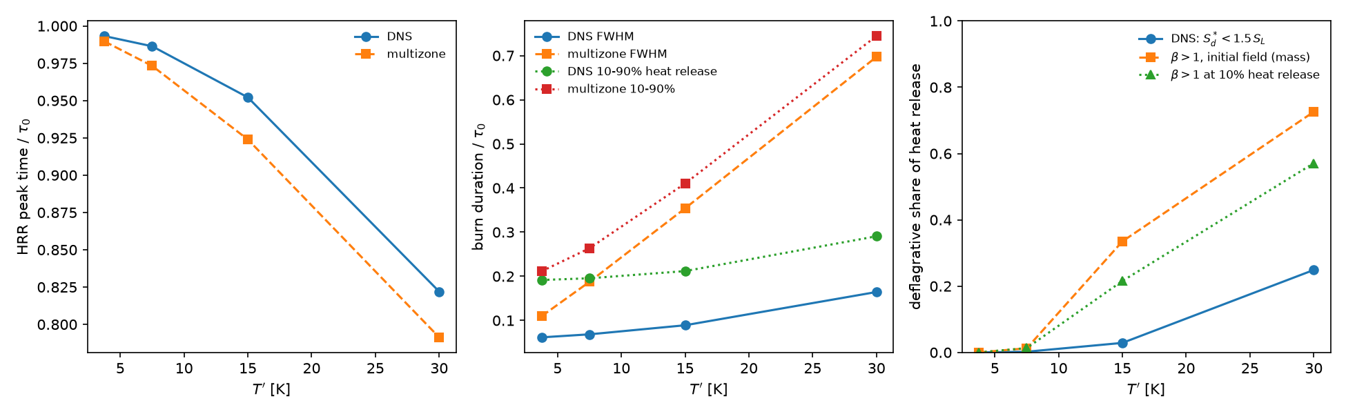
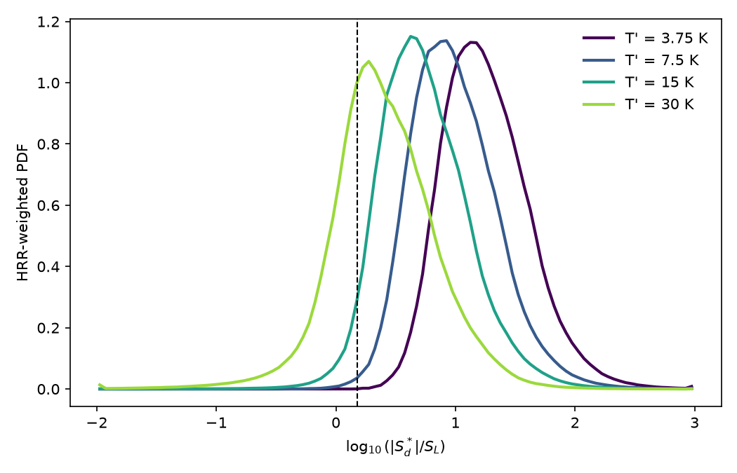
As the papers describe, larger fluctuations ignite earlier and burn longer, and the fronts slow from spontaneous ignition towards deflagration. The comparison is qualitative: the papers' figures were not available for a quantitative one, and they used another H₂ mechanism.

• Multizone model: without transport, it predicts bursts 2–4 times wider than the DNS. Turbulent mixing halves T′ before ignition (at T′ = 15 K, to 8.5 K by 0.45 τ₀), and deflagrations consume the coldest gas.
• β criterion: Sankaran et al.'s criterion marks a larger part of the mixture as deflagrative than the DNS front speeds show (figure above).
• Threshold: the deflagrative share depends on the threshold. At T′ = 30 K it is 15%, 25% and 51% at 1.1, 1.5 and 3 S_L, but the shift of the front-speed distribution with T′ does not depend on it.

Large-eddy simulation

Mallard's large-eddy simulation (#203, #205, #213, #214, #215, #222, #223, #230, #224; guide, design notes). The LES uses:

• an explicit eddy-viscosity model, Sigma (Nicoud et al. 2011) by default. In 3D, its filter width is the cell-volume width with the anisotropy correction of Scotti, Meneveau & Lilly (1993), the default since #223;
• the hybrid convective flux: kinetic-energy-preserving and central, with the Riemann solver only where a compression sensor fires;
• MUSCL without a limiter.

The kinetic-energy budget of [integrals] measures how much of the dissipation comes from the model, the scheme and molecular viscosity. That tells explicit LES, where the model does the work, from implicit LES, where the scheme does. Each case also runs without the model and with HLLC at every face.

Decaying isotropic turbulence

d8060fd with the uncommitted files of #213 (0.5.0 + 83 commits on the LES branch). The dynamic constant: development code between 0.6.0 and 0.7.0 (#223)

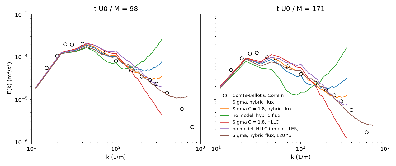
The grid turbulence of Comte-Bellot & Corrsin (1971), in the cbc_les example. A periodic box of eleven mesh lengths starts from the measured spectrum at the first station (t U₀/M = 42). The spectra are compared at the next two stations, 98 and 171, with a fictitious sound speed for a turbulent Mach number of 0.1. Spectral error is the log₁₀ RMS of E_LES/E_CBC up to 2/3 of the grid cutoff wavenumber, at stations 2 / 3. The dissipation shares are averaged over the run.

Energy spectra at t U₀/M = 98 and 171 against Comte-Bellot & Corrsin: Sigma with the hybrid flux, without a model, and with HLLC.

Mesh	Flux	Model	Spectral error	Numerical / SGS share of dissipation
64³	hybrid	Sigma	0.107 / 0.104	1.3 / 69.1%
64³	hybrid	Sigma, C = 1.8	0.058 / 0.063	1.3 / 79.6%
64³	hybrid	none	0.226 / 0.375	−7.7 / 0%
64³	HLLC	Sigma, C = 1.8	0.154 / 0.217	46.3 / 43.5%
64³	HLLC	none (implicit LES)	0.135 / 0.114	83.8 / 0%
128³	hybrid	Sigma	0.063 / 0.085	2.0 / 52.2%
128³	hybrid	none	0.182 / 0.249	1.8 / 0%

• Hybrid flux: the model does the work, and the scheme's share is 1–2% at every resolution. Without the model, energy piles up at the grid cutoff, and the spectral error is 2–4 times larger.
• HLLC at every face: the scheme does 84% of the dissipation without a model, and still 46% with one. Such runs are implicit LES whatever the model.
• Model constant: the best Sigma constant depends on the resolution, 1.8 at 64³ and the literature's 1.35 (the default) at 128³. The opt-in dynamic procedure sets C to 1.6, 1.4 and 1.15 at 32³, 64³ and 128³. It gives the best spectra of any run at 128³ (0.060 / 0.054), but not the 1.8 that fits 64³.
• Budget: these shares were measured before #222 redefined the numerical dissipation from the scheme's own discrete pressure work. For non-reacting flows the change is small: at 64³ with C = 1.8 the numerical share goes from 0.7% to −0.9%.

Turbulent channel flow, Re_τ = 395 and 590

Cell-volume width at Re_τ = 395: the #214 branch around the 0.6.0 release (commit not recorded). Scotti's width, the dynamic constant and Re_τ = 590: development code between 0.6.0 and 0.7.0 (#223, #230)

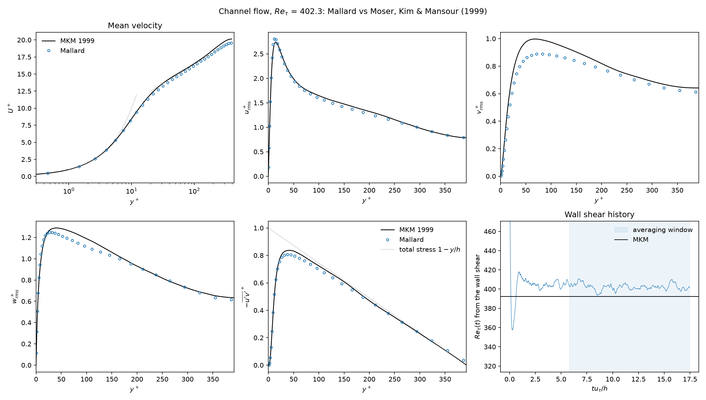
Wall-resolved LES of the channel at Re_τ = 395 against Moser, Kim & Mansour (1999), in the channel_les example. The box is 2πh × 2h × πh with 64³ hexahedra: Δx⁺ 39, Δz⁺ 19, Δy⁺ 0.9 at the wall. The mass flow is held at the DNS's bulk Reynolds number, with resolved fluctuations averaged over t = 100–300 h/U_b. MKM's Re_τ at this bulk Reynolds number is 392.2.

Re_τ = 395: mean velocity, resolved RMS velocities and Reynolds shear stress against MKM (Sigma with the cell-volume width, 64³), and Re_τ(t) from the wall shear.

Mesh	Flux	Model	Reτ	Cf	numerical / SGS / molecular dissipation
64³	hybrid	Sigma, Scotti width (default)	+0.7%	+0.9%	not reported
64³	hybrid	Sigma, cell-volume width	402.3 (+2.6%)	+4.8%	3.5 / 12.6 / 83.9%
64³	hybrid	Sigma, C = 1.8	389.4 (−0.7%)	−1.9%	2.8 / 16.6 / 80.6%
64³	hybrid	none	420.1 (+7.1%)	+14.2%	5.0 / 0 / 95.0%
64³	HLLC	Sigma, C = 1.8	317.6 (−19%)	−35%	13.5 / 5.4 / 81.1%
48³	hybrid	Sigma, C = 1.8	381.3 (−2.8%)	−5.9%	3.2 / 17.9 / 78.9%

• Model on, 64³: Re_τ is within 3% at both Sigma constants and with either filter width, and the mean velocity is within 3% across y⁺ = 30–300. Scotti's width brings Re_τ from +2.6% to +0.7%. The opt-in dynamic constant (C = 1.09) gives +4.0%, worse than the static one.
• Model off: Re_τ is 7% high, more than twice the error with the model.
• Resolved stresses: the resolved u_rms, w_rms and −u′v′ are within 10%. The resolved v_rms peak is 11–15% low (see 590 below).
• HLLC instead of the hybrid flux: the scheme removes 2.5 times as much energy as the model. Re_τ is then 19% low.
• Refinement: the error with the model decreases from 48³ to 64³.

At Re_τ = 590 (input_590.toml, MKM's Re_τ 587.2), the numerics of the 395 case run on 96³ hexahedra: Δx⁺ 38, Δz⁺ 19, Δy⁺ 0.87. Statistics are averaged over t = 60–200 h/U_b.

Re_τ = 590: profiles against MKM (Sigma with Scotti's width, the default), and Re_τ(t).

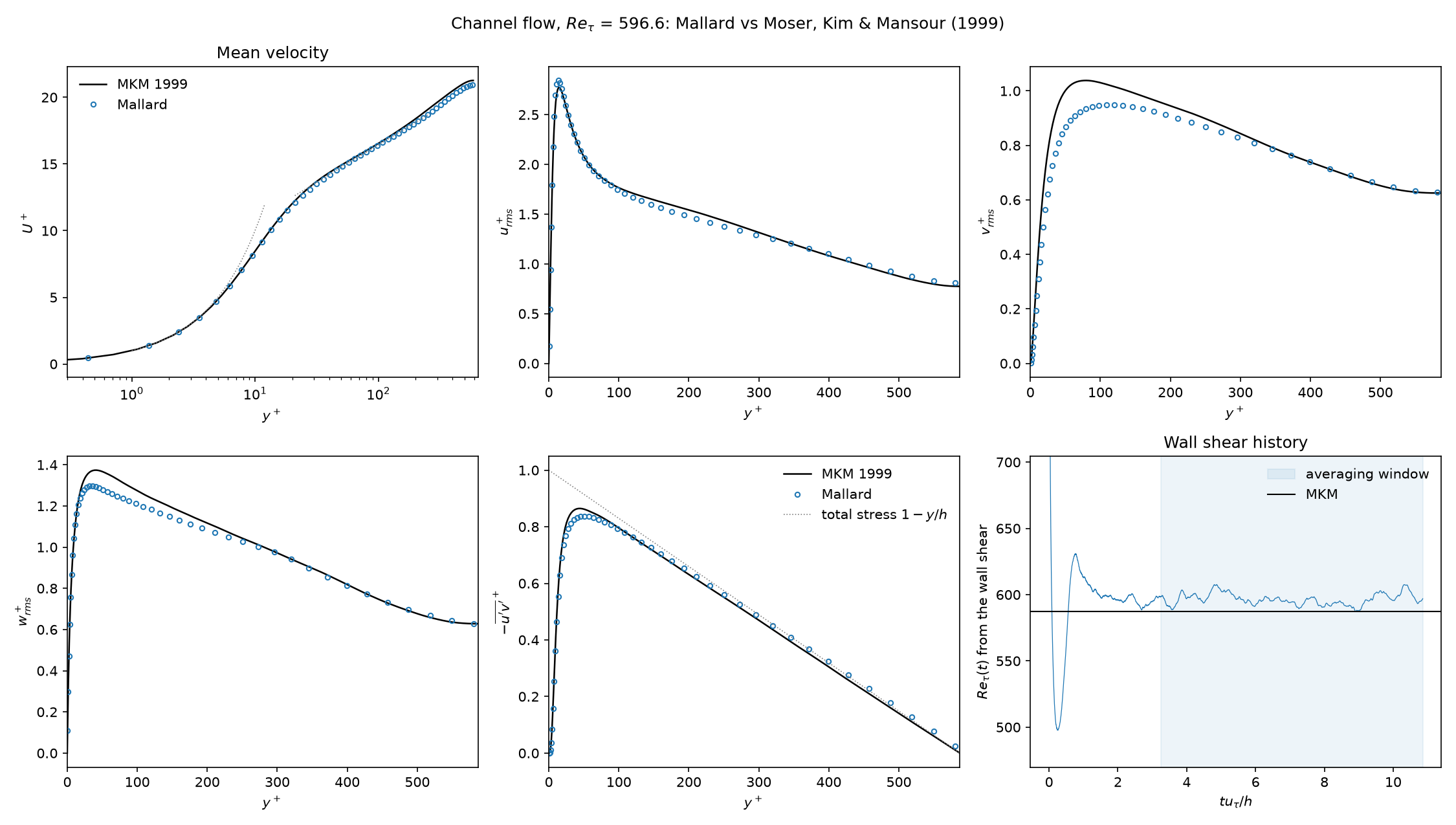
Model	Reτ	Cf	peak vrms+ (MKM 1.04)	numerical / SGS / molecular dissipation
Sigma, Scotti width (default)	596.6 (+1.6%)	+2.9%	0.95	3.3 / 16.2 / 80.6%
Sigma, cell-volume width	611.0 (+4.1%)	+7.9%	0.96	2.3 / 13.5 / 84.2%
none	632.7 (+7.8%)	+15.7%	1.02	3.3 / 0 / 96.7%

• Scotti's width: the targets hold at 590. Re_τ is within 3%, the mean profile within 2% for y⁺ = 30–100, and u_rms, w_rms and −u′v′ within 10%.
• Cell-volume width: the model halves the model-off error but misses the Re_τ target.
• v_rms: the resolved peak is 8–9% low at 590, and 8% low at 395 on a mesh with Δx⁺ 26 and Δz⁺ 13. It barely depends on the model, so it is the streamwise and spanwise resolution of the near-wall cycle.

Bluff-body combustor, non-reacting

The branch of #252 (version string 0.6.0; commit not recorded), merged as 83c961c; first released in Mallard 0.8.0

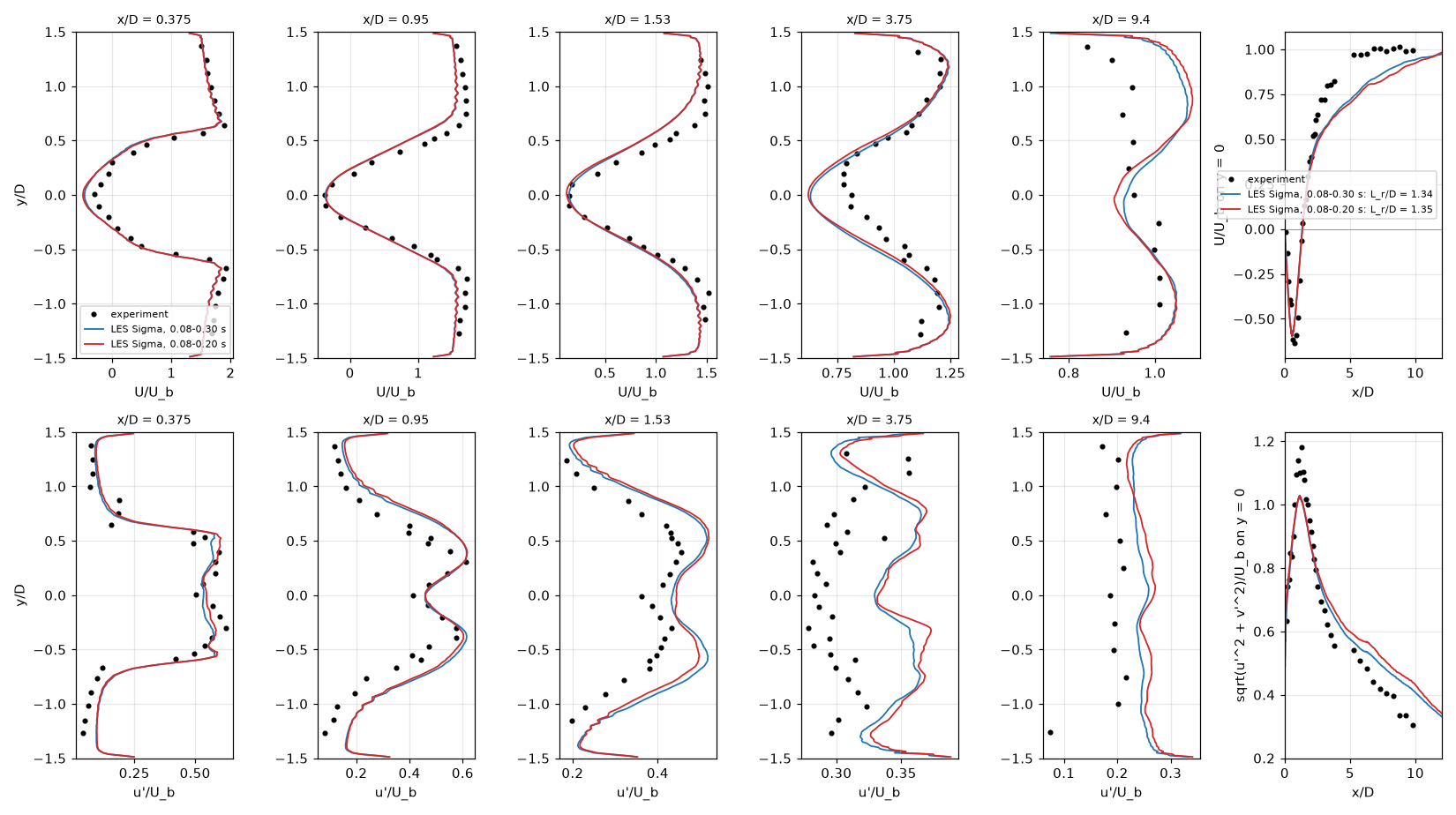
The cold flow of the Volvo bluff-body combustor (Sjunnesson et al.) in the volvo_bluff_body example (cold.toml), against the experiment's LDA data.

• Numerics: Sigma model with Scotti's width, the hybrid flux, MUSCL.
• Mesh and boundaries: 2.7 million hexahedra (Δ = D/32) with a periodic span, digital-filter inflow at 5% and a characteristic outlet.
• Statistics: over 0.08–0.30 s, 26 shedding periods; 626,000 steps at 14 ms on four A100 GPUs.

Q-criterion isosurfaces behind the triangular bluff body, over the streamwise velocity on a back plane.

Mean (top) and RMS (bottom) streamwise velocity at x/D = 0.375–9.4 and along the centerline, against Sjunnesson et al.'s measurements.

Quantity	LES	Experiment
recirculation length Lr/D	1.34	1.35
centerline minimum of U/Ub	−0.59 at x/D = 0.61	−0.64 at 0.75
mean |ΔU|/Ub at x/D = 0.375 / 0.95 / 1.53 / 3.75 / 9.4	0.13 / 0.14 / 0.11 / 0.07 / 0.08
Strouhal number	0.285
εnum/εSGS	−0.38

Caveat: the dissipation budget gives ε_num/ε_SGS = −0.38. The scheme feeds resolved energy back at 38% of the subgrid model's rate, steadily in every 40 ms window. No model-off run was made. The reacting case (reacting.toml) is set up but not validated: its thickening must stay at F ≤ 5, which needs 15–28 million cells.

Thickened flame

5741305 with the uncommitted files of #215 (0.6.0 + 6 commits)

The dynamically thickened flame model (TFLES; Colin et al. 2000), with Charlette et al.'s (2002) efficiency function, on a one-dimensional stoichiometric H₂/air flame. Cantera gives s_L = 2.3324 m/s and δ_L = 0.330 mm; MUSCL with HLLC.

Mesh	Thickening F	Consumption speed	Displacement speed	Thermal thickness
2 cells per δL	7.91	2.327 m/s (−0.2%)	2.291 m/s (−1.8%)	2.615 mm (F δL = 2.610 mm)
0.5 cells per δL	31.6	2.328 m/s (−0.2%)	2.251 m/s (−3.5%)
0.5 cells per δL, no model	1	2.273 m/s (−2.5%)	2.240 m/s (−4.0%)	one cell

The thickened flame keeps the laminar flame speed with the thickness F δ_L it is designed to have. Without the model, the flame's structure is one cell wide, set by the scheme.

Premixed flame in decaying turbulence

Development code between 0.6.0 and 0.7.0, the branch of #222 (from a172f6f)

A stoichiometric H₂/air flame in decaying turbulence, in the flame_turbulence example.

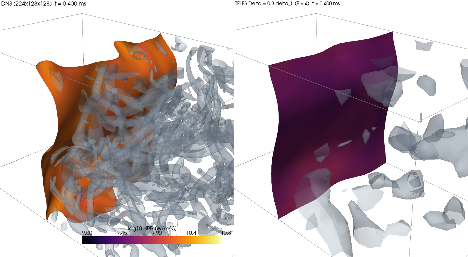
• DNS reference: 224 × 128 × 128 cells of δ_L/10, u′ = 2.1 S_L, Karlovitz number 2, numerical dissipation 0.4%.
• LES: TFLES with the Sigma model, on the same initial field box-filtered to Δ = 0.4, 0.8 and 1.6 δ_L (thickening F = 2, 4, 8).
• Measured: the turbulent flame speed S_T, from the rate at which the fresh gas is consumed, over 0.2–0.4 ms. The DNS gives S_T/S_L = 1.132.

The DNS: the flame surface colored by heat release rate, and the turbulent eddies ahead of it in the fresh gas.

The DNS (left) and TFLES at Δ = 0.8 δ_L (right) at t = 0.4 ms.

Δ / δL	TFLES, Colin efficiency (default)	TFLES, eddy_viscosity subgrid velocity	TFLES, E = 1	quasi-laminar
0.4	1.056 (−6.7%)	1.065 (−5.9%)	1.050 (−7.2%)	1.088 (−3.9%)
0.8	1.053 (−6.9%)	1.034 (−8.6%)	0.985 (−13%)	1.166 (+3.0%)
1.6	2.240 (+98%)	1.008 (−11%)	0.947 (−16%)	1.051 (−7.1%)

Turbulent flame speed, fuel consumption speed and flame surface over time, and temperature distributions in the flame brush: DNS and LES variants.

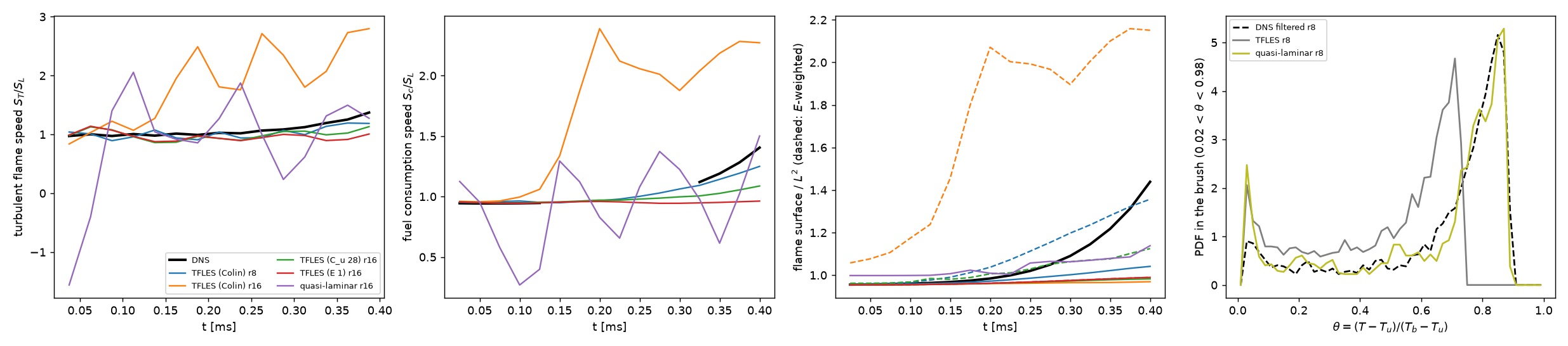
• TFLES with the default efficiency is within 10% of the DNS for Δ ≤ 0.8 δ_L. It is smooth in time, and the scheme's dissipation is at most 20% of the model's.
• Δ = 1.6 δ_L: Colin's subgrid-velocity operator overshoots and doubles the flame speed. On the filtered DNS its subgrid velocity is 5–8 times the DNS's.
• Second turbulent field: an independent case, not used for any calibration, shows the same doubling.
• The opt-in eddy_viscosity subgrid velocity removes the overshoot. Its constant is calibrated on this case and is not independently validated.
• Quasi-laminar runs, without a flame model, get a close mean speed on coarse meshes. They are erratic in time (33–36% rms) and up to 15% numerically dissipated.

Non-premixed flame in turbulence: PaSR (experimental)

Development code between 0.6.0 and 0.7.0, the branches of #222 and #224

Experimental

The partially stirred reactor closure ([les.combustion] model = "pasr", #224) is an opt-in, not a default. It helps at moderate filter widths and overcorrects on coarse meshes.

PaSR scales the chemical rates of each cell by κ = τ_c / (τ_c + τ_mix). The chemical time comes from the heat release, and the mixing time from the filter width and the molecular plus eddy viscosity.

• DNS reference: an H₂/N₂ (25% H₂) against air diffusion flame, started from a counterflow profile (strain 160 1/s), in the box and decaying turbulence of the premixed case, to 0.4 ms. The DNS temperature at the stoichiometric surface is 1262 K.
• LES: Sigma model at Δ = 0.27 and 0.53 mm (8 and 16 DNS cells), with PaSR and with quasi-laminar chemistry, i.e. the filtered state's rates without a combustion model.
• Measured: the heat release over 0.2–0.4 ms, against the DNS.

Δ	PaSR	quasi-laminar
0.27 mm	−10.7% (κ 0.62 at the stoichiometric surface)	+16.6%
0.53 mm	−50% (Tst 892 K, near extinction; κ 0.26)	+41%

• Finer width: PaSR moves the heat release the right way.
• Coarser width: it overcorrects. The mixing time τ_mix = Δ²/(ν + ν_t), with the constant C_mix = 1, is overestimated, and the flame comes spuriously close to extinction.
• Budget: |ε_num/ε_SGS| ≤ 0.10 with PaSR, 0.23 quasi-laminar.

References

The sources of the reference data and test cases on this page. The sources of the numerical methods themselves, with where Mallard uses each, are on the References page.

• F. S. Billig, Shock-wave shapes around spherical- and cylindrical-nosed bodies, J. Spacecraft Rockets 4, 822–823 (1967). doi:10.2514/3.28969
• M. E. Brachet, D. I. Meiron, S. A. Orszag, B. G. Nickel, R. H. Morf and U. Frisch, Small-scale structure of the Taylor–Green vortex, J. Fluid Mech. 130, 411–452 (1983).
• F. Charlette, C. Meneveau and D. Veynante, A power-law flame wrinkling model for LES of premixed turbulent combustion. Part I: non-dynamic formulation and initial tests, Combust. Flame 131, 159–180 (2002). doi:10.1016/S0010-2180(02)00400-5
• J. H. Chen, E. R. Hawkes, R. Sankaran, S. D. Mason and H. G. Im, Direct numerical simulation of ignition front propagation in a constant volume with temperature inhomogeneities: I. Fundamental analysis and diagnostics, Combust. Flame 145, 128–144 (2006). doi:10.1016/j.combustflame.2005.09.017
• O. Colin, F. Ducros, D. Veynante and T. Poinsot, A thickened flame model for large eddy simulations of turbulent premixed combustion, Phys. Fluids 12, 1843–1863 (2000). doi:10.1063/1.870436
• G. Comte-Bellot and S. Corrsin, Simple Eulerian time correlation of full- and narrow-band velocity signals in grid-generated, 'isotropic' turbulence, J. Fluid Mech. 48, 273–337 (1971). doi:10.1017/S0022112071001599
• G. S. Constantinescu and K. D. Squires, LES and DES investigations of turbulent flow over a sphere at Re = 10,000, Flow Turbul. Combust. 70, 267–298 (2003). doi:10.1023/B:APPL.0000004937.34078.71
• V. Daru and C. Tenaud, Numerical simulation of the viscous shock tube problem by using a high resolution monotonicity-preserving scheme, Computers & Fluids 38, 664–676 (2009).
• R. Deiterding, High-resolution numerical simulation and analysis of Mach reflection structures in detonation waves in low-pressure H₂–O₂–Ar mixtures: a summary of results obtained with the adaptive mesh refinement framework AMROC, J. Combust. 2011, 738969 (2011). doi:10.1155/2011/738969
• R. P. Fedkiw, B. Merriman and S. Osher, High accuracy numerical methods for thermally perfect gas flows with chemistry, J. Comput. Phys. 132, 175–190 (1997). doi:10.1006/jcph.1996.5622
• B. Franzelli, E. Riber, L. Y. M. Gicquel and T. Poinsot, Large Eddy Simulation of combustion instabilities in a lean partially premixed swirled flame, Combust. Flame 159, 621–637 (2012). doi:10.1016/j.combustflame.2011.08.004
• D. G. Goodwin, R. L. Speth, H. K. Moffat and B. W. Weber, Cantera: an object-oriented software toolkit for chemical kinetics, thermodynamics, and transport processes, version 3.2.0, cantera.org.
• J.-F. Haas and B. Sturtevant, Interaction of weak shock waves with cylindrical and spherical gas inhomogeneities, J. Fluid Mech. 181, 41–76 (1987). doi:10.1017/S0022112087002003
• E. R. Hawkes, R. Sankaran, P. P. Pébay and J. H. Chen, Direct numerical simulation of ignition front propagation in a constant volume with temperature inhomogeneities: II. Parametric study, Combust. Flame 145, 145–159 (2006). doi:10.1016/j.combustflame.2005.09.018
• E. Johnsen, J. Larsson, A. V. Bhagatwala, W. H. Cabot, P. Moin, B. J. Olson, P. S. Rawat, S. K. Shankar, B. Sjögreen, H. C. Yee, X. Zhong and S. K. Lele, Assessment of high-resolution methods for numerical simulations of compressible turbulence with shock waves, J. Comput. Phys. 229, 1213–1237 (2010). doi:10.1016/j.jcp.2009.10.028
• T. A. Johnson and V. C. Patel, Flow past a sphere up to a Reynolds number of 300, J. Fluid Mech. 378, 19–70 (1999). doi:10.1017/S0022112098003206
• A. Keating, U. Piomelli, E. Balaras and H.-J. Kaltenbach, A priori and a posteriori tests of inflow conditions for large-eddy simulation, Phys. Fluids 16, 4696–4712 (2004). doi:10.1063/1.1811672
• J. Kim, D. Kim and H. Choi, An immersed-boundary finite-volume method for simulations of flow in complex geometries, J. Comput. Phys. 171, 132–150 (2001). doi:10.1006/jcph.2001.6778
• M. Klein, A. Sadiki and J. Janicka, A digital filter based generation of inflow data for spatially developing direct numerical or large eddy simulations, J. Comput. Phys. 186, 652–665 (2003). doi:10.1016/S0021-9991(03)00090-1
• C. Liu, X. Zheng and C. H. Sung, Preconditioned multigrid methods for unsteady incompressible flows, J. Comput. Phys. 139, 35–57 (1998).
• P. J. Martínez Ferrer, R. Buttay, G. Lehnasch and A. Mura, A detailed verification procedure for compressible reactive multicomponent Navier–Stokes solvers, Computers & Fluids 89, 88–110 (2014). doi:10.1016/j.compfluid.2013.10.014
• R. D. Moser, J. Kim and N. N. Mansour, Direct numerical simulation of turbulent channel flow up to Re_τ = 590, Phys. Fluids 11, 943–945 (1999). doi:10.1063/1.869966
• F. Nicoud, H. Baya Toda, O. Cabrit, S. Bose and J. Lee, Using singular values to build a subgrid-scale model for large eddy simulations, Phys. Fluids 23, 085106 (2011). doi:10.1063/1.3623274
• E. S. Oran, J. W. Weber, E. I. Stefaniw, M. H. Lefebvre and J. D. Anderson, A numerical study of a two-dimensional H₂-O₂-Ar detonation using a detailed chemical reaction model, Combust. Flame 113, 147–163 (1998). doi:10.1016/S0010-2180(97)00218-6
• J. Park, K. Kwon and H. Choi, Numerical solutions of flow past a circular cylinder at Reynolds numbers up to 160, KSME Int. J. 12, 1200–1205 (1998).
• T. Poinsot, D. Veynante and S. Candel, Quenching processes and premixed turbulent combustion diagrams, J. Fluid Mech. 228, 561–606 (1991). doi:10.1017/S0022112091002823
• J. J. Quirk, A contribution to the great Riemann solver debate, Int. J. Numer. Methods Fluids 18, 555–574 (1994).
• R. Sankaran, H. G. Im, E. R. Hawkes and J. H. Chen, The effects of non-uniform temperature distribution on the ignition of a lean homogeneous hydrogen–air mixture, Proc. Combust. Inst. 30, 875–882 (2005). doi:10.1016/j.proci.2004.08.176
• A. Scotti, C. Meneveau and D. K. Lilly, Generalized Smagorinsky model for anisotropic grids, Phys. Fluids A 5, 2306–2308 (1993). doi:10.1063/1.858537
• Sjunnesson, Henrikson & Löfström, AIAA Paper 92-3650 (1992), doi:10.2514/6.1992-3650; the LDA data as digitized from Wu et al. (2017), arXiv:1707.05805.
• L. I. Sedov, Similarity and Dimensional Methods in Mechanics, Academic Press (1959).
• J. E. Shepherd, Shock and Detonation Toolbox, Explosion Dynamics Laboratory, Caltech, shepherd.caltech.edu/EDL/PublicResources/sdt.
• C.-W. Shu, Essentially non-oscillatory and weighted essentially non-oscillatory schemes for hyperbolic conservation laws, in Advanced Numerical Approximation of Nonlinear Hyperbolic Equations, Lecture Notes in Mathematics 1697, 325–432 (1998).
• C.-W. Shu and S. Osher, Efficient implementation of essentially non-oscillatory shock-capturing schemes, II, J. Comput. Phys. 83, 32–78 (1989).
• G. P. Smith, D. M. Golden, M. Frenklach, N. W. Moriarty, B. Eiteneer, M. Goldenberg, C. T. Bowman, R. K. Hanson, S. Song, W. C. Gardiner, V. V. Lissianski and Z. Qin, GRI-Mech 3.0, combustion.berkeley.edu/gri-mech.
• G. A. Sod, A survey of several finite difference methods for systems of nonlinear hyperbolic conservation laws, J. Comput. Phys. 27, 1–31 (1978).
• A. Subramaniam, M. L. Wong and S. K. Lele, A high-order weighted compact high resolution scheme with boundary closures for compressible turbulent flows with shocks, J. Comput. Phys. 397, 108822 (2019). doi:10.1016/j.jcp.2019.07.021
• G. I. Taylor, The formation of a blast wave by a very intense explosion. I. Theoretical discussion, Proc. R. Soc. Lond. A 201, 159–174 (1950). doi:10.1098/rspa.1950.0049
• A. G. Tomboulides, S. A. Orszag and G. E. Karniadakis, Direct and large-eddy simulation of the flow past a sphere, in Engineering Turbulence Modelling and Experiments 2, Elsevier, 273–282 (1993). doi:10.1016/B978-0-444-89802-9.50030-7
• E. F. Toro, Riemann Solvers and Numerical Methods for Fluid Dynamics, 3rd ed., Springer (2009).
• N. Tsuboi, S. Katoh and A. K. Hayashi, Three-dimensional numerical simulation for hydrogen/air detonation: rectangular and diagonal structures, Proc. Combust. Inst. 29, 2783–2788 (2002). doi:10.1016/S1540-7489(02)80339-X
• D. N. Williams, L. Bauwens and E. S. Oran, Detailed structure and propagation of three-dimensional detonations, Proc. Combust. Inst. 26, 2991–2998 (1996). doi:10.1016/S0082-0784(96)80142-1
• C. H. K. Williamson, Vortex dynamics in the cylinder wake, Annu. Rev. Fluid Mech. 28, 477–539 (1996).
• H. Wu, P. C. Ma and M. Ihme, the SIMPLER balanced splitting, Comput. Phys. Commun. (2019). doi:10.1016/j.cpc.2019.04.016
• G. Zhou, K. Xu and F. Liu, Grid-converged solution and analysis of the unsteady viscous flow in a two-dimensional shock tube, Phys. Fluids 30, 016102 (2018), doi:10.1063/1.4998300; arXiv:1705.09062.