Documentation of the main branch

These pages follow Mallard's main branch, which is ahead of release 0.8.0: some features they describe come with the next release.

Large-eddy simulation

With an [les] table (type = "navier_stokes", planar runs), Mallard solves the filtered equations with an explicit eddy-viscosity model of the subgrid scales (SGS). This chapter gives the filtered equations, the four SGS models, the filter width, the global dynamic procedure, the two turbulent combustion models (thickened flame and partially stirred reactor) and the synthetic turbulence of characteristic inlets. The low-dissipation convective flux used with LES is in chapter 6. Usage: Large-eddy simulation; design and validation: LES design notes.

Filtered equations

With a spatial filter \(\overline{\phi}\) of width \(\Delta\) and the Favre filter \(\widetilde{\phi} = \overline{\rho\phi}/\overline{\rho}\), Mallard solves eq. (2) of chapter 1 for \(\overline{\rho}\), \(\overline{\rho}\widetilde{\mathbf{u}}\), \(\overline{\rho}\widetilde{E}\) and \(\overline{\rho}\widetilde{Y}_k\), with the molecular fluxes evaluated at the filtered state and the unclosed SGS fluxes modelled by gradient-diffusion closures:

\[ \begin{equation} \boldsymbol{\tau}^\mathrm{sgs} = 2\mu_t\,\widetilde{\mathbf{S}}^d, \qquad \mathbf{q}^\mathrm{sgs} = -\lambda_t\nabla\widetilde{T}, \quad \lambda_t = \frac{c_p\,\mu_t}{Pr_t}, \qquad \mathbf{j}_k^\mathrm{sgs} = -\frac{\mu_t}{Sc_t}\frac{W_k}{\overline{W}}\nabla\widetilde{X}_k + \widetilde{Y}_k\sum_j\frac{\mu_t}{Sc_t}\frac{W_j}{\overline{W}}\nabla\widetilde{X}_j, \label{eq:filtered-equations} \end{equation} \]

with \(\widetilde{\mathbf{S}}^d = \tfrac12(\nabla\widetilde{\mathbf{u}} + \nabla\widetilde{\mathbf{u}}^T) - \tfrac13(\nabla\cdot\widetilde{\mathbf{u}})\mathbf{I}\) and \(\mu_t = \overline{\rho}\,\nu_t\) (src/solver/solver_les.cpp). That is, \(\mu_t\) is added to \(\mu\) in eq. (5) of chapter 1, \(\lambda_t\) to \(\lambda\), and for mixtures \(\overline{\rho}\,\nu_t/Sc_t\) to every \(\rho D_k\) of eq. (10) of chapter 2, so the SGS species fluxes keep the correction velocity and sum to zero. \(Pr_t\) = Pr_t and \(Sc_t\) = Sc_t (both default 0.9). The isotropic part of the SGS stress, the SGS diffusion of kinetic energy and the subgrid parts of the molecular fluxes are neglected, and without a combustion model the filtered reaction rates are those of the filtered state. Wall faces keep the molecular fluxes only (chapter 8). The eddy viscosity is recomputed at every stage from the cell velocity gradients of the viscous terms (chapter 5); filter symbols are dropped in the other chapters.

Subgrid-scale models

Each model is an eddy viscosity

\[ \begin{equation} \nu_t = (C\Delta)^2\,\mathcal{D}(\mathbf{g}) \quad \text{(Smagorinsky, WALE, Sigma)}, \qquad \nu_t = c\,\Delta^2\,\mathcal{D}(\mathbf{g}) \quad \text{(Vreman)}, \label{eq:subgrid-scale-models-1} \end{equation} \]

of the resolved velocity gradient \(g_{ij} = \partial\widetilde{u}_i/\partial x_j\), taken as that of a three-dimensional flow with \(u_z = \partial_z = 0\) in 2D builds (src/physics/les.h). With \(\mathbf{S} = \tfrac12(\mathbf{g} + \mathbf{g}^T)\) and \(\mathbf{A} : \mathbf{B} = A_{ij}B_{ij}\), the operators \(\mathcal{D}\) and the default constants ([les] model, C) are

• Smagorinsky (Smagorinsky 1963; Lilly's constant \(C_s = 0.17\)):

  \[ \begin{equation} \mathcal{D} = \sqrt{2\,\mathbf{S}:\mathbf{S}}; \label{eq:subgrid-scale-models-2} \end{equation} \]

• WALE (Nicoud & Ducros 1999; \(C_w = 0.5\)), with \(\mathbf{S}^g\) the traceless symmetric part of \(\mathbf{g}^2\):

  \[ \begin{equation} \mathcal{D} = \frac{(\mathbf{S}^g:\mathbf{S}^g)^{3/2}}{(\mathbf{S}:\mathbf{S})^{5/2} + (\mathbf{S}^g:\mathbf{S}^g)^{5/4}}, \qquad S^g_{ij} = \tfrac12\left(g_{ik}g_{kj} + g_{jk}g_{ki}\right) - \tfrac13\delta_{ij}\,g_{kl}g_{lk}; \label{eq:subgrid-scale-models-3} \end{equation} \]

• Vreman (Vreman 2004; \(c = 0.07\)), with \(\alpha_{ij} = \partial\widetilde{u}_j/\partial x_i\) and \(\beta_{ij} = \alpha_{mi}\alpha_{mj}\):

  \[ \begin{equation} \mathcal{D} = \sqrt{\frac{B_\beta}{\alpha_{ij}\alpha_{ij}}}, \qquad B_\beta = \beta_{11}\beta_{22} - \beta_{12}^2 + \beta_{11}\beta_{33} - \beta_{13}^2 + \beta_{22}\beta_{33} - \beta_{23}^2; \label{eq:subgrid-scale-models-4} \end{equation} \]

• Sigma (Nicoud et al. 2011; \(C_\sigma = 1.35\); the default in 3D), with \(\sigma_1 \ge \sigma_2 \ge \sigma_3 \ge 0\) the singular values of \(\mathbf{g}\):

  \[ \begin{equation} \mathcal{D} = \frac{\sigma_3\,(\sigma_1 - \sigma_2)(\sigma_2 - \sigma_3)}{\sigma_1^2}. \label{eq:subgrid-scale-models-5} \end{equation} \]

  \(\sigma_1^2\) is the largest eigenvalue of \(\mathbf{G} = \mathbf{g}^T\mathbf{g}\) from the trigonometric solution of its characteristic cubic (Nicoud et al., appendix); \(\sigma_2^2\) and \(\sigma_3^2\) follow from \(\sigma_2^2 + \sigma_3^2 = (I_2 - \sigma_2^2\sigma_3^2)/\sigma_1^2\) and \(\sigma_2^2\sigma_3^2 = \det(\mathbf{g})^2/\sigma_1^2\), with \(I_2\) the second invariant of \(\mathbf{G}\), which keeps them accurate when small (\(\sigma_3 = 0\) exactly for planar gradients). Sigma vanishes for every 2D flow, so 2D builds reject it and default to WALE.

Filter width

The filter width is the cell size \(\Delta_V = \lvert\Omega_i\rvert^{1/d}\) (filter_width = "volume", the default in 2D) or, in 3D, that size corrected for the cell's anisotropy as Scotti, Meneveau & Lilly 1993 propose ("scotti", the default in 3D):

\[ \begin{equation} \Delta = \Delta_V\cosh\sqrt{\tfrac{4}{27}\left((\ln a_1)^2 - \ln a_1\ln a_2 + (\ln a_2)^2\right)}, \qquad a_1 = \frac{h_1}{h_3},\ a_2 = \frac{h_2}{h_3}. \label{eq:filter-width} \end{equation} \]

The extents \(h_1 \le h_2 \le h_3\) of an arbitrary cell are \(h_m = \lvert\Omega_i\rvert/\lambda_m\), with \(\lambda_m\) the eigenvalues of its projected-area tensor \(\tfrac12\sum_f A_f\,\mathbf{n}_f\mathbf{n}_f^T\) (exact for boxes, equal for regular tetrahedra).

Global dynamic procedure

With dynamic = true, the model constant is computed once per time step from the Germano identity over the whole domain (Germano et al. 1991; Lilly 1992; Favre-weighted as in Moin et al. 1991; DynamicProcedureFunctor). The test filter \(\widehat{\phi}\) of a cell is the volume-weighted average over the cell and its vertex neighbors, of width

\[ \begin{equation} \widehat{\Delta}^2 = \Delta^2 + \frac{12}{d}\,\mathrm{tr}\,\mathrm{cov}(\mathbf{x}), \label{eq:global-dynamic-procedure-1} \end{equation} \]

where \(\mathrm{cov}(\mathbf{x})\) is the volume-weighted covariance of the stencil's centroids (\(\widehat{\Delta} = 3\Delta\) on uniform hexahedra). Filtered gradients stand for the gradients of the filtered field. With the model written as \(\boldsymbol{\tau}^{\mathrm{sgs},d} = -2\,C^2\,\overline{\rho}\,\Delta^2\,\mathcal{D}(\mathbf{g})\,\widetilde{\mathbf{S}}^d\) (Vreman: \(c\) for \(C^2\)),

\[ \begin{equation} \mathbf{L} = \widehat{\overline{\rho}\widetilde{\mathbf{u}}\widetilde{\mathbf{u}}} - \frac{\widehat{\overline{\rho}\widetilde{\mathbf{u}}}\,\widehat{\overline{\rho}\widetilde{\mathbf{u}}}}{\widehat{\overline{\rho}}}, \qquad \mathbf{M} = 2\left(\widehat{\overline{\rho}\,\Delta^2\mathcal{D}(\mathbf{g})\,\widetilde{\mathbf{S}}^d} - \widehat{\overline{\rho}}\,\widehat{\Delta}^2\,\mathcal{D}(\widehat{\mathbf{g}})\,\widehat{\mathbf{S}}^d\right), \label{eq:global-dynamic-procedure-2} \end{equation} \]

\[ \begin{equation} C^2 = \max\left(0,\ \frac{\langle\mathbf{L}^d:\mathbf{M}\rangle}{\langle\mathbf{M}:\mathbf{M}\rangle}\right), \label{eq:global-dynamic-procedure-3} \end{equation} \]

with \(\langle\cdot\rangle\) the volume integral over all owned cells, summed in fixed point so that the constant is bitwise independent of the number of ranks. A field without resolved strain (\(\langle\mathbf{M}:\mathbf{M}\rangle = 0\)) keeps the previous constant.

Thickened flame model

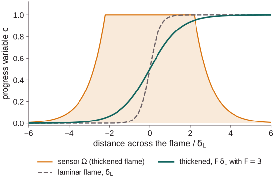
[les.combustion] model = "tfles" resolves a premixed flame thinner than the mesh by thickening it (Colin et al. 2000; Légier et al. 2002; Butler & O'Rourke 1977; src/physics/tfles.h). From the laminar flame's thermal thickness \(\delta_L\) and speed \(s_L\) (delta_L, s_L) and its unburnt and burnt temperatures (T_unburnt, T_burnt), each cell has a flame sensor, a thickening factor and an efficiency:

\[ \begin{equation} \Omega = \min\left(1,\ \frac{c\,(1 - c)}{c_0\,(1 - c_0)}\right), \quad c = \min\left(1, \max\left(0, \frac{T - T_u}{T_b - T_u}\right)\right), \quad c_0 = 0.05, \label{eq:thickened-flame-model-1} \end{equation} \]

\[ \begin{equation} F = 1 + (F_\mathrm{max} - 1)\,\Omega, \qquad F_\mathrm{max} = \max\left(1,\ \frac{n_\mathrm{res}\,\Delta_V}{\delta_L}\right), \label{eq:thickened-flame-model-2} \end{equation} \]

with \(n_\mathrm{res}\) = n_res (default 5) cells across the thickened flame. Within the flame, the molecular conductivity and diffusivities (thermal diffusion included) are multiplied by \(\mathcal{E}F\) and the reaction rates by \(\mathcal{E}/F\), so that the flame is \(F\) times thicker and propagates at \(\mathcal{E}s_L\); the SGS heat and species fluxes are multiplied by \(1 - \Omega\), since the thickened flame is resolved. The rate multiplier is applied by integrating each cell's chemistry over \((\mathcal{E}/F)\,\tau\) (chapter 3).

The efficiency \(\mathcal{E}\) restores the flame surface that thickening removes from the subgrid wrinkling. With efficiency = "dynamic" (the default) it is the saturated power law of Charlette, Meneveau & Veynante 2002 at the filter width \(\Delta_e = F\delta_L\), with an exponent from the dynamic procedure of Wang, Boileau & Veynante 2011:

\[ \begin{equation} \mathcal{E} = F^{\beta}, \qquad \beta = \frac{\ln\left(\sum_c \widehat{\lvert\nabla c\rvert}\,V_c \big/ \sum_c \lvert\nabla\widehat{c}\rvert\,V_c\right)} {\sum_c \ln\gamma_c\,\lvert\nabla\widehat{c}\rvert\,V_c \big/ \sum_c \lvert\nabla\widehat{c}\rvert\,V_c}, \qquad \gamma_c^2 = 1 + \frac{n\,\widehat{\Delta}_c^2}{(F_{max}\delta_L)^2}, \label{eq:dynamic-efficiency} \end{equation} \]

from the identity that the total flame surface is the same seen at the combustion filter and at the test filter, \(\langle \mathcal{E}_{\Delta_e}\lvert\nabla c\rvert\rangle = \langle \mathcal{E}_{\gamma\Delta_e}\lvert\nabla\widehat{c}\rvert\rangle\). \(c\) is the sensor's progress variable and gradients are least squares on the vertex-neighbor stencil. The test filter \(\widehat{\cdot}\) is \(n\) passes of the volume average over the cell and its vertex neighbors, each of squared width \(\widehat{\Delta}_c^2 = (12/d)\,\mathrm{tr}(\mathrm{cov})\) of the stencil's centroids (\(8h^2\) on cubes of side \(h\)); \(n\), fixed at setup, is the smallest that makes \(n\widehat{\Delta}^2\) reach \((F_{max}\delta_L)^2\) on average over the thickened cells (4 on cubes at \(n_{res} = 5\), \(\gamma = 1.51\)). The sums run over the owned cells with \(F_{max} > 1\) and are exact in fixed point, so \(\beta\) does not depend on the rank count; \(\beta\) is clipped to \([0, 1]\), and is 0 when the resolved surface \(\sum_c\lvert\nabla\widehat{c}\rvert V_c\) is below \(10^{-6}\sum_c V_c/\Delta_e\) (no flame). With efficiency = "charlette" it is their efficiency function of a subgrid velocity at the filter width \(F\delta_L\):

\[ \begin{equation} \mathcal{E} = \left(1 + \min\left[F - 1,\ \Gamma\frac{u'_\Delta}{s_L}\right]\right)^{\beta}, \label{eq:thickened-flame-model-3} \end{equation} \]

with \(\beta\) = beta (default 0.5) and

\[ \begin{equation} \begin{aligned} \Gamma &= \left[\left(f_u^{-a} + f_\Delta^{-a}\right)^{b/a} + f_{Re}^{-b}\right]^{-1/b}, \qquad a = 0.6 + 0.2\,e^{-0.1\,u'_\Delta/s_L} - 0.2\,e^{-0.01F}, \quad b = 1.4, \\ f_u &= 4\sqrt{\frac{27C_k}{110}}\,\frac{18C_k}{55}\left(\frac{u'_\Delta}{s_L}\right)^2, \qquad f_\Delta = \sqrt{\frac{27C_k\pi^{4/3}}{110}\left(F^{4/3} - 1\right)}, \qquad f_{Re} = \sqrt{\frac{9}{55}\exp\left(-\frac{3C_k\pi^{4/3}}{2\,Re_\Delta}\right)}\,\sqrt{Re_\Delta}, \end{aligned} \label{eq:thickened-flame-model-4} \end{equation} \]

\(C_k = 1.5\) and \(Re_\Delta = u'_\Delta F\delta_L/\nu\) (\(\nu\) the molecular kinematic viscosity). The SGS velocity is Colin et al.'s operator, which ignores dilatation (subgrid_velocity = "colin", the default), or a multiple of the eddy viscosity ("eddy_viscosity"):

\[ \begin{equation} u'_\Delta = 2\,\Delta_V^3\left\lvert\nabla^2(\nabla\times\widetilde{\mathbf{u}})\right\rvert \qquad\text{or}\qquad u'_\Delta = C_u\,\frac{\nu_t}{\Delta_V}, \label{eq:thickened-flame-model-5} \end{equation} \]

with \(C_u\) = C_u (default 28). The Laplacian of the vorticity is the divergence of its face gradients, cell gradients averaged to interior faces and corrected along the line of centroids as the viscous fluxes are (chapter 6); boundary faces carry none. Without the efficiency (efficiency = "none") or where \(F = 1\) or \(u'_\Delta = 0\), \(\mathcal{E} = 1\). The fields \(\Omega\), \(F\) and \(\mathcal{E}\) are evaluated once per time step and held over its stages.

Partially stirred reactor

[les.combustion] model = "pasr" scales each cell's reaction rates, those of its filtered state, by the reacting fraction of the partially stirred reactor (Sabelnikov & Fureby 2013; src/physics/pasr.h):

\[ \begin{equation} \kappa = \frac{\tau_c}{\tau_c + \tau_\mathrm{mix}}, \qquad \tau_c = \frac{\rho\,c_p\,T}{\lvert\dot\omega_T\rvert}, \qquad \tau_\mathrm{mix} = C_\mathrm{mix}\frac{\Delta_V^2}{\nu + \nu_t}, \label{eq:partially-stirred-reactor} \end{equation} \]

with \(\dot\omega_T\) the heat release rate of eq. (2) of chapter 3 at the filtered state, \(C_\mathrm{mix}\) = C_mix (default 1) and the cell size \(\Delta_V\). As the mesh resolves the mixing (\(\Delta_V \to 0\)), \(\kappa \to 1\); where the chemistry is fast, the rate tends to the mixing-limited \(\kappa\dot\omega \approx \dot\omega\,\tau_c/\tau_\mathrm{mix}\). \(\kappa\) is evaluated once per time step and applied as the rate multiplier of the chemistry substeps.

Synthetic inflow turbulence

A characteristic inlet (nscbc_inlet) with a [boundaries.turbulence] table imposes a target velocity \(\mathbf{u}^\mathrm{t} = \overline{\mathbf{u}} + \mathbf{u}'\) per face, whose fluctuation comes from the digital filter of Klein, Sadiki & Janicka 2003 with the Reynolds stress imposed as Lund, Wu & Squires 1998 propose (src/boundary/synthetic_inflow.cpp). How the target enters the flow is in chapter 8.

1. Random field. Independent unit-variance random numbers \(r_j(\mathbf{k}, m)\) for each velocity component \(j\) live on an auxiliary uniform grid on the inlet plane, one plane per generator time step \(\Delta t_p\). They come from a counter-based hash of (seed, inlet, component, grid point, plane index), so the field at a given time does not depend on the number of ranks, on the time steps taken or on restarts.

2. Filter. Each component is filtered with Gaussian kernels along the two transverse directions and in time, Klein's third direction by Taylor's hypothesis with the convection velocity \(U_c\) (convection_velocity, default the area-mean inflow speed). For an integral length of \(n\) grid spacings (or planes) the kernel is

   \[ \begin{equation} b_k = \frac{\exp\left(-\pi k^2/(2n^2)\right)}{\left(\sum_{l=-N}^{N}\exp\left(-\pi l^2/n^2\right)\right)^{1/2}}, \qquad \lvert k\rvert \le N = \lceil 2n\rceil, \label{eq:synthetic-inflow-turbulence-1} \end{equation} \]

   normalized to \(\sum_k b_k^2 = 1\), so that the filtered field has unit variance and the two-point correlation \(\exp(-\pi r^2/(4n^2))\), whose integral is \(n\) spacings. The length scales \(L_{j,d}\) (length_scale) set \(n\) per component and direction; the grid spacing is the smallest transverse length divided by points_per_length (default 6), and \(\Delta t_p = L_\mathrm{stream}/(n_p\,U_c)\) likewise, with \(n_p\) = points_per_length and \(L_\mathrm{stream}\) the smallest streamwise length. On periodic directions the grid wraps and the half width is capped at what fits in a period. 3. Interpolation. Face centroids interpolate the filtered planes bilinearly in space and linearly in time, and divide by the exact standard deviation of the interpolated value (from the correlation \(\rho_1\) of neighboring grid points), so that every face's fluctuation \(\mathbf{v}\) has unit variance. 4. Reynolds stress. With \(\mathbf{R}\) the Reynolds stress of the inlet (reynolds_stress, or from a profile of plane averages) and \(\mathbf{L}_R\) its lower Cholesky factor,

   \[ \begin{equation} \mathbf{u}' = \mathbf{L}_R\,\mathbf{v}, \qquad \mathbf{L}_R\mathbf{L}_R^T = \mathbf{R}. \label{eq:synthetic-inflow-turbulence-2} \end{equation} \]

3. Zero net flux. With zero_net_flux = true (the default), the area mean of the normal fluctuation over the whole inlet is subtracted, so the inlet's mean mass flow is not perturbed.