Design: inlets

Status: implemented (stagnation_inlet, mass_flow_inlet, numbers as expressions of x, y, z, t).

upt imposes velocity, pressure and temperature, which over-specifies a subsonic inflow: one characteristic, the acoustic wave travelling upstream, leaves the domain through it. Nozzles, ducts and intakes need inlets that impose only what the flow upstream sets and take the rest from the interior.

At a subsonic inflow face, with u the velocity along the inward normal, four kinds of wave meet (five in 3D):

• λ = u: entropy, the tangential velocity and the composition, entering;
• λ = u + c: the incoming acoustic wave, entering;
• λ = u − c: the outgoing acoustic wave, from the interior.

An inlet imposes all but the last. Like every Mallard boundary, it does so weakly: it builds a ghost state from the interior face state, and the Riemann solver takes the flux between the two.

stagnation_inlet

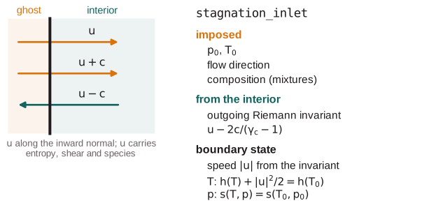
The inlet imposes the stagnation temperature T0, the stagnation pressure p0, the flow direction d (by default the inward normal of each face) and, for mixtures, the composition. The interior supplies the outgoing Riemann invariant, which fixes the speed V = |u|:

J(W) = u_n + 2 c / (γ_c − 1),   c² = γ_c p / ρ     (u_n along the outward normal)
J(W_ghost) = J(W_interior),    u_ghost = V d
h(T) + V² / 2 = h(T0)          (energy)
s(T, p) = s(T0, p0)            (isentrope, at fixed composition)

For a calorically perfect gas, h = cp T and p / p0 = (T / T0)^(γ / (γ − 1)), and γ_c = γ: this is the classical subsonic inflow condition (e.g. Blazek, ch. 8).

For a thermally perfect mixture, the ghost state lies on the mixture's own isentrope. h(T) is the mixture enthalpy from the NASA polynomials, and at fixed composition

ln(p / p0) = (s°(T) − s°(T0)) / R

where s° is the mixture's standard-state entropy without the mixing term, which cancels at fixed composition (ThermoTable::s0_mass). A constant ratio of specific heats would put the state elsewhere. For air at T0 = 2500 K, the frozen γ(T0) misses the true isentrope by more than 0.1% in pressure already 300 K below T0. The unit tests integrate the isentrope from cp(T) alone and check that a state on it is a fixed point of the inlet.

Only the invariant uses a constant γ_c, the frozen ratio at T0. It is the same function of the state on both sides, so an interior state on the isentrope is reproduced exactly, for any γ(T). It only decides which point of the isentrope is taken, not the total conditions.

J(V) is monotone along the isentrope. The solver brackets T in [10⁻³ T0, T0] and runs a safeguarded Newton iteration in double precision (about five iterations); for mixtures each iteration evaluates h and cp of the inlet composition.

Special cases:

• Outflow, or an interior above p0. If J exceeds that of the stagnation state (2 c0 / (γ_c − 1)), the ghost is the stagnation state at rest. The Riemann solver then lets the flow out against p0.
• Supersonic inflow (u_n ≤ −c). Every wave enters, and none is left to fix the speed. The ghost keeps the interior speed, at T0, p0 and d.
• Supersonic outflow. The ghost is the interior state.

Reconstruction and the other paths

The ghost depends on the interior state, as farfield's does:

• Flux. The face's reconstructed interior state goes in.
• Gradients and TENO's mirror cells. These take the cell's own state. The solve then stays out of every kernel but the flux's: computing the ghost there too, even in runs without the inlet, slowed the 3D TENO5 benchmark by a third. A uniform flow that is the inlet's own state stays exact.
• Mixtures. The inflow carries the inlet's composition in the species fluxes and their reconstruction. The ghost's frozen [γ, e0] are those at the ghost temperature. The surrogates in the scalar reconstruction stay the cell's own, since they vary with the ghost.
• Viscous terms. Viscous fluxes treat the inlet like upt: the cell's values and gradients.

Verification

test/inlet_test.cpp checks:

• Fixed point. A perfect-gas interior on the isentrope at Mach 0.02, 0.3 and 0.8 is reproduced to round-off, along the normal and oblique to it.
• Conservation laws. For an interior off the isentrope: the total enthalpy and the isentrope hold, the outgoing invariant is preserved, and the flow follows d. The backflow and supersonic cases are covered too.
• Thermally perfect fixed point. The same holds for air at T0 = 2500 K on its true isentrope, which a constant γ misses.
• Equivalence with a perfect gas. A one-species constant-cp mixture gives the perfect-gas flow to round-off.
• Uniform duct. Thermally perfect air from T0 = 2000 K, p0 = 2 bar to a 1.4 bar outlet, with MUSCL and TENO, settles at the exact isentropic exit state: velocity within 0.02%, temperature within 0.002%.
• Nozzle. The converging-diverging nozzle below, on a coarse mesh.
• MPI. A distributed run matches the serial one.

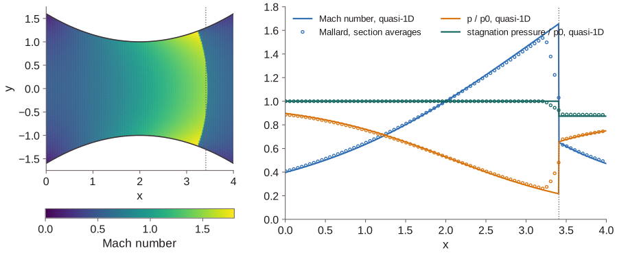
The nozzle example is a planar converging-diverging nozzle with inlet and exit 1.6 throat heights, fed at p0, T0. The back pressure 0.75 p0 puts a normal shock in the diverging part. examples/nozzle/plot_nozzle.py compares the section averages with the quasi-one-dimensional solution (--figure redraws this figure):

	Mallard (320 × 20)	Quasi-1D
Mass flow / choked	0.9983	1
Shock position (section-averaged pressure)	3.384 (2 cells upstream)	3.409
Stagnation pressure ahead of the shock	1 ± 5e-4	1
Stagnation pressure ratio across the shock	0.886	0.874

The mass flow sits below the choked one because the sonic line of a planar nozzle is curved; the quasi-1D theory has it straight. The shock is curved too (it stands further upstream at the wall), and its section average is weaker than the quasi-1D one: 1.4% less loss of stagnation pressure, which moves it two cells upstream.

mass_flow_inlet

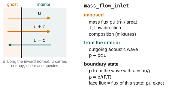
The inlet imposes the mass flux G = ρ u · n_in, the temperature T, the flow direction d and the composition. The interior supplies the outgoing acoustic wave, linearized about the interior state:

p + Z u_n = p_i + Z u_n,i,    Z = sqrt(γ_c p_i ρ_i)       (u_n along the outward normal)
u_n = −G / ρ = −G R T / p
⇒ p² − (p_i + Z u_n,i) p − Z G R T = 0                     (the positive root)
ρ = p / (R T),   u = G / (ρ |d · n|) d

γ_c is the condition's own frozen ratio of specific heats at T for mixtures (the gas's γ otherwise). The pressure is a closed form, with no iteration.

The flux is the boundary state's. A ghost state alone does not hold the mass flow. The Riemann flux between the interior state and a ghost of mass flux G carries G only where the two states agree. Heat release or compression behind the inlet keeps them apart, and the mass flow drifts with them. The face flux is therefore the physical flux of the boundary state: the Riemann solver gets the boundary state on both sides, and every solver returns F(W_b) for equal states. Its mass flux is ρ u · n = −G to round-off, at every quadrature point. Species enter at G Y_k. With double flux, both sides use the cell's frozen thermodynamics, as at any face.

The pressure still comes from the interior, so the face keeps the outgoing acoustic wave's characteristic relation. A boundary-state flux is stable where a single wave leaves, which is the subsonic inflow this condition is for.

mdot is divided among the faces by profile × face measure, summed over the faces of owned cells on all ranks. The faces' total is then mdot exactly, with whatever measure the flux integral uses (per unit depth in 2D, r L per radian in axisymmetric runs). A face with a mass flux of its own (an expression, or a profile) gets its own copy of the condition, as the faces of a composition that varies along upt do.

An NSCBC-relaxed variant, relaxing the mass flux like nscbc_inlet relaxes the velocity, would let acoustic waves leave; it is not implemented. mass_flow_inlet reflects them like upt, at a fixed mass flux instead of a fixed velocity.

Verification

test/inlet_test.cpp:

• Ghost. The ghost carries G, T and d, and keeps the outgoing acoustic wave, for interior densities from 0.5 to 3.
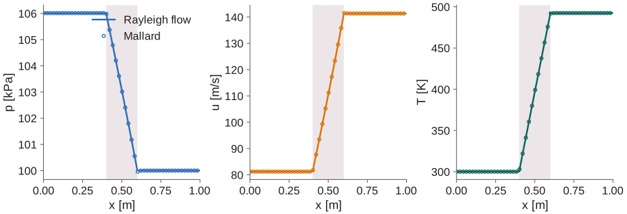
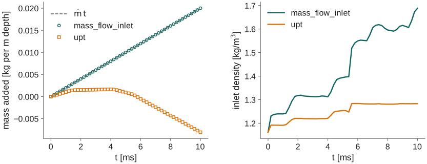
• Closed heated duct. A duct closed at the far end and heated in its middle gains exactly mdot t (to 1e-11 of it, in practice 1e-14). This holds for a single gas with MUSCL/HLLC and TENO/Roe, for mixtures with and without double flux, and for a uniform mass_flux as well as an mdot with a profile. upt at the same initial mass flux misses by more than 1%.
• Rayleigh flow. Steady flow through a heated duct to a pressure outlet matches Rayleigh flow to 1e-4: the inlet pressure the flow needs, and the exit velocity and temperature.
• MPI. An mdot with a profile on two to four ranks matches the serial run.

examples/heated_duct (examples/heated_duct/plot_heated_duct.py):

• Steady duct. On 200 cells, the inlet pressure is within 1e-5 and the exit temperature within 1e-6 of Rayleigh flow.
• Closed duct. The mass added stays within 1.1e-14 of mdot t while the inlet density rises from 1.16 to 1.69 kg/m³. With upt, the duct first gains less, then loses gas through the inlet once its pressure exceeds the inlet's.

Numbers as expressions of x, y, z and t

The inflow numbers (u, p, T of upt and nscbc_inlet, p0, T0, mass_flux), the wall velocity and the mixture composition may be expressions (BoundaryFields, src/boundary/boundary_fields.h).

• Per face. A condition with an expression gets a copy for each of its faces, as composition profiles already did, holding the values at the face center.
• Per stage. The expressions are compiled (expr::Program). Copies with expressions of t are re-evaluated by one kernel at each stage time (TimedBoundaryFields), which reads the time from the device scalar stage_time, so the step's CUDA graph replays it. For mixtures the kernel also sets the composition, gas constant, frozen [gamma, e0] and the transport values. nscbc_inlet's velocity goes into its faces' targets: at the stage time, and at the end of the step for the target's own incoming wave (TimedInletTargets).
• Cost. Time-independent inputs are evaluated once, and nothing runs per stage for them. Time-dependent ones cost one small kernel per stage and keep the CUDA graph (mixtures and characteristic boundaries step without one anyway).
• Range. A device flag records the first number of t out of its range (face, time, value); the host checks it at each progress check and before reporting a divergence, and stops with an input error.

test/inlet_test.cpp (ForcedInletTest) checks the stage times. With SSPRK3 on a fixed mesh, a temporal-refinement study (steps dt and dt / 2 against dt / 8, forcing at 40 rad/s with dt = 0.0075, and at 20 rad/s with dt = 0.004 for nscbc_inlet) converges at:

Forced input	Order
upt T(t)	2.75
upt u(t)	2.91
stagnation_inlet p0(t)	3.00
mass_flow_inlet mass_flux(t)	2.91
moving wall u(t)	3.02
nscbc_inlet u(t)	1.20

The same study gives 1.21 to 1.28 if the inputs are taken at the start of each step instead of at the stage times. In single precision the moving wall's errors reach round-off; the test then checks that they fall to it. nscbc_inlet is first order either way: its boundary point advances by a forward-Euler step of the LODI relation once per step.