Probes and monitors
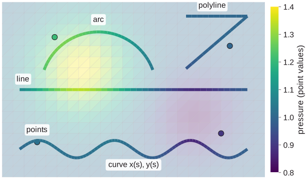
Probes sample the solution where you choose: at points, along curves, on cut planes and surfaces, over boundary zones and over regions. Monitors reduce the solution to a few numbers per output: the force on a wall and integrals over the domain. Each writes its own files (What a run writes), with units and provenance.
Probes: [[probes]]
A probe samples the solution on a geometry every interval steps (or
time_interval of simulation time) and writes the samples, reductions over
them, or both; a probe of a region writes integrals, means and
extrema over it. The files are the same bit for bit on any number of ranks.
On a GPU the files have the CPU's rows, in the same order, with the same steps,
times, coordinates, normals, areas and region volumes: the geometry and the
region fractions are set up on the host, and rank 0 reduces the gathered samples
(cells, for a region) on the host in sample order. The values agree
with a CPU run to rounding, not bit for bit, since the device rounds the solution
and its point values differently (fused multiply-adds, its own math functions).
The test suite checks every backend against a CPU reference (test/data/probes):
indices, steps and times exactly, geometry to 1e-14 and values to 1e-10 of each
column's largest magnitude. The geometry tolerance covers other CPUs and
compilers only; on one host the geometry of every backend is the same bit for bit.
[[probes]]
name = "centerline"
variables = ["RHO", "P"]
start = [0.0, 0.01]
end = [1.0, 0.01]
n_points = 200
interval = 10
Used in: pulsed_jet, source_regions, cylinder, channel_inflow_retau180, turbulent_inflow_duct and 2 more.
# Wake survey: high-order point values on an arc, a VTK series for ParaView,
# and the arc's mean and RMS in probe_wake_reductions.csv
[[probes]]
name = "wake"
variables = ["U", "P"]
sampling = "point"
type = "arc"
center = [0.0, 0.0]
radius = 5.0
angles = [-45.0, 45.0]
n_points = 91
time_interval = 1.0
format = "vtp"
reductions = ["mean", "rms"]
| Key | Default | Meaning |
|---|---|---|
name |
required | Names the files |
variables |
required | [statistics] fields; U and Y_* expand to all components and species |
type |
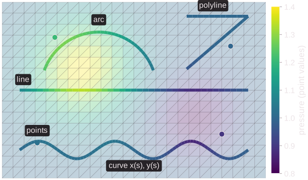
from the keys | point, points (points or points_file), line, polyline, circle, arc, curve (x, y, z of s), cut_plane (point, normal, optional bounds); 3D surface (x, y, z of u, v) |
region |
none | Instead of type: a region or its name, reduced over its cells (below) |
sampling |
cell |
cell: the average of the cell holding each sample; point: the reconstruction's value at the sample |
interval / time_interval |
1 step | Output times; time_interval shortens the step to land on them |
format |
csv |
csv, hdf5 (one extensible file), vtkhdf (one VTKHDF file of every output, which ParaView opens as a time series) or vtp (one file per output and a .pvd series) |
reductions |
none (region: integral, mean, min, max) |
integral, mean, favre, min, max, rms over the geometry |
samples |
true |
false writes only the reductions |
scale, rotate, pivot, translate |
none | Move the geometry (scale, then rotate, about pivot, then translate) |
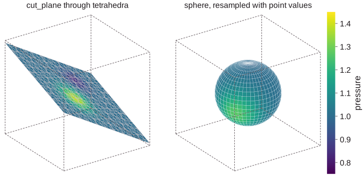
Cut planes and surfaces
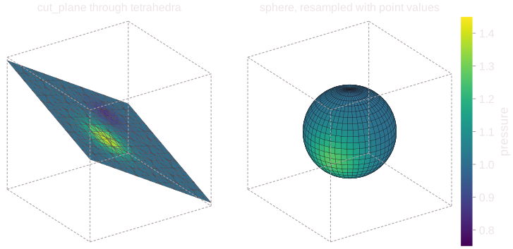
type = "cut_plane" intersects the mesh exactly with a plane: one sample per
cut cell, and integrals exact for the reconstruction polynomials. Surfaces
are regions, resampled on a grid with n_points:
region = {type = "sphere", center = [0.5, 0.5, 0.5], radius = 0.3, filled = false}
with n_points = [24, 48]. Both have normals, so fluxes through them are
variables: a closed sphere's integral of MASS_FLUX is the net outflow.
[[probes]]
name = "midplane"
type = "cut_plane"
point = [0.0, 0.0, 0.5]
normal = [0.0, 0.0, 1.0]
variables = ["U", "P", "MASS_FLUX"]
sampling = "point"
format = "vtp"
time_interval = 0.01
reductions = ["integral"]
Boundary data
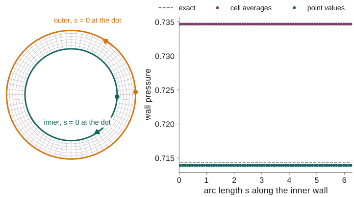
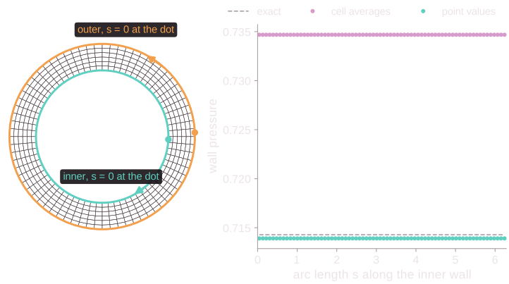
boundary = "<zone>" (a name or a list) or boundary_type = "wall" (every
wall) turns each face of the zones into a sample: the state the boundary
condition sets on the face, wall quantities and fluxes. In 2D the faces form
ordered polylines with their arc length s; in 3D, polygons for ParaView.
[[probes]]
name = "cylinder"
boundary = "cylinder"
variables = ["P", "CP", "CF", "Q_W", "Y_PLUS"]
reference = {rho = 1.0, u = [0.2, 0.0], p = 0.7142857142857143}
time_interval = 1.0

[[probes]]
name = "inflow"
boundary = ["inlet", "outlet"]
samples = false
variables = ["MASS_FLUX", "MOMENTUM_FLUX", "ENTHALPY_FLUX"]
reductions = ["integral"]
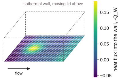
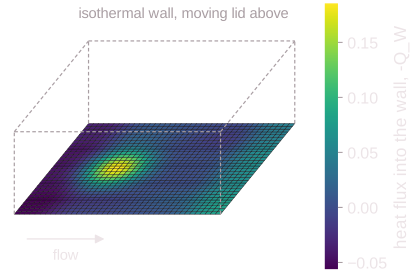
In 3D the faces are polygons; ParaView colors the .vtp series by any variable:
| Variable | Meaning |
|---|---|
MASS_FLUX, MOMENTUM_FLUX, ENTHALPY_FLUX, SPECIES_FLUX_* |
Convective fluxes through the face, positive out of the domain |
TRACTION_PRESSURE, TRACTION_VISCOUS |
Force per unit area on the boundary; their integral is the [[forces]] force (per radian in axisymmetric runs, as area) |
TAU_W, TAU_W_X, ... |
Wall shear stress (magnitude, components) |
CF, CP |
Skin friction and pressure coefficients of reference |
Q_W |
Heat flux into the fluid |
U_TAU, Y_PLUS |
Friction velocity and first-cell y+ |
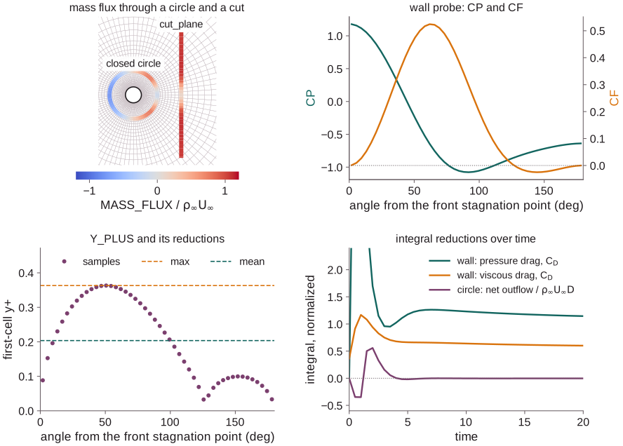
Around a cylinder at Re = 40: the wall probe's CP, CF and Y_PLUS, the
mean and max of Y_PLUS, the integral of the tractions (the drag) and
the MASS_FLUX through a closed circle and a cut, whose net outflow settles
to zero:
Accuracy and pitfalls
With TENO, sampling = "point" reads each cell's reconstruction polynomial at
the sample, so a probe converges at the scheme's order (fifth order for
order = 5) instead of the first order of cell averages at points off the
centroids. The Sod comparison on the Numerics
page was read from a line probe. The full key list is in the input reference;
each type, where its samples go and how to read the files, with figures:
Geometry.
Pitfalls:
- Point values fall back to the linear least-squares reconstruction in cells the TENO indicator flags troubled (shocks, and coarse meshes of smooth fields), and to the cell average outside the domain.
- Mass fractions are cell averages in both modes;
TandHfollow the reconstructedp / rhoat the cell's composition. - CSV is for small probes: it repeats the coordinates every output. Use
vtkhdf,hdf5orvtpfor thousands of samples. - Wall shear and heat flux use the viscous flux's one-sided wall gradients:
second-order shear on smooth meshes, first-order heat flux at isothermal
walls.
CFis signed alongreference.u. - A cut plane is exact for the mesh's straight-sided cells (curved cells are
cut as their straight versions);
boundsclips it to a box. - Fluxes of boundary probes are those of the face states, not the scheme's numerical fluxes: they agree as the mesh is refined.
- Reductions of points weigh each point 1 (
integralis a sum); curves integrate with three Gauss points per element between samples.
Region probes
# Mass, mean temperature and pressure range in a box, every 10 steps
[[probes]]
name = "box"
variables = ["RHO", "T", "P"]
region = {type = "rectangle", center = [0.5, 0.5], size = [0.4, 0.2]}
reductions = ["integral", "mean", "min", "max"]   # the default
interval = 10
Used in: source_regions.
A probe with region reduces the cell averages of the cells the region covers,
each weighted by its volume times its volume fraction f, so a region need not
follow the mesh: integral is sum f V q (the mass in the region for RHO),
mean that over sum f V, favre the density-weighted mean, rms the root
mean square, and min, max the extremes over the cells with f > 0. Rank 0
sums them in global cell order, so they are the same bit for bit on any number
of ranks. The region may be one of the mesh's own: region = "domain" gives
the totals of the whole domain (the mass, for RHO), a cell zone those of its
cells (regions of the mesh). A surface,
curve or set of points weighs each cell by its area, length or count in the
cell instead of f V (on a mesh):
integral is then the surface integral, mean the area-weighted mean,
evaluated at the elements' quadrature points (cell averages, or point values
with sampling = "point"), and the third column is area, length or
count. Surfaces (2D: curves) have normals, so their fluxes (MASS_FLUX, ...)
are variables too: a closed surface's integral of MASS_FLUX is the net
outflow. Each output
appends a row to reductions_file (default probe_<name>_reductions.csv):
The third column is sum f V: volume in 3D and axisymmetric runs (per
radian), area in planar 2D runs (per unit depth). Give the region by name to
measure exactly where a source or sponge acts:
[regions]
heater = {type = "sphere", center = [0, 0, 0], radius = 0.01, edge = 0.002}

[[sources]]
rhoE = "1 MW/m^3"
region = "heater"

[[probes]]
name = "heater"
variables = ["T"]
region = "heater"
Pitfalls:
- Values are cell averages, so
minandmaxare those of the cells, not of the field inside them, and include cells the region only touches. - A region probe has no samples:
type,sampling,format,fileandsamplesdo not apply to it.
Wall forces: [[forces]]
Used in: sphere_mach3, sphere_axisymmetric, cylinder, sphere_re300, channel_retau180 and 2 more.
Writes step, t and the pressure and viscous force components of the fluid
on the zone, per unit depth in 2D (per radian in axisymmetric runs). Divide by
the dynamic pressure and a reference length (or area) for drag and lift
coefficients. On walls with a wall model
the viscous force is the modeled stress, and a last column Q gives the
modeled heat flux into the fluid.
Domain integrals: [integrals]
Used in: taylor_green_3d, isotropic_turbulence, channel_retau180, forced_isotropic_turbulence, cbc_les and 4 more.
Writes integrals.csv with the volume integrals of the kinetic energy,
enstrophy, squared dilatation and pressure dilatation, and of |u|^2,
|omega|^2, rho^2, T and T^2 (from which mean squares and variances
follow). For decaying turbulence (the Taylor–Green
vortex) the dissipation rate is -dE/dt. With TENO, velocity gradients come
from the reconstruction polynomials (order-consistent: within 1% of spectral
derivatives of the same field). budget = true adds the
kinetic-energy budget:
molecular, SGS and numerical dissipation.
See also
- Input reference:
[[probes]],[[forces]],[integrals] - Geometry: probe types, sample placement, reading probe files
- Statistics: time averages, spectra and phase averages
- Output: snapshots, the run record (which repeats the latest forces and integrals at each progress row), units and file formats