Wall models

A wall boundary with a wall_model table takes its shear stress and heat flux from a model of the inner layer instead of from the resolved velocity and temperature gradients at the wall. This chapter gives the exchange point that feeds the model, the two models (the equilibrium ODE model and the inverse-velocity-transformation model of Griffin, Fu & Moin), how their output replaces the wall's viscous flux, and what that implies for parallel runs and restarts (src/physics/wall_model.h, src/boundary/wall_exchange.h, src/boundary/wall_exchange.cpp). Usage: Large-eddy simulation; design and validation: wall model design notes.

Wall-modeled LES

A wall-resolved LES (chapter 4) places its first cell at \(y^+ \approx 1\), so the cell count of a wall-bounded flow grows like \(Re_\tau^2\) (Choi & Moin 2012). Wall-modeled LES (WMLES) resolves only the outer part of the boundary layer, with cells that scale with its thickness \(\delta\): the near-wall layer is left to a model that returns the wall shear stress \(\tau_w\) and the heat flux into the fluid \(q_w\) from the LES state at a height \(h\) above the wall (Larsson et al. 2016; Bose & Park 2018). In wall units, with \(u_\tau = \sqrt{\tau_w/\rho_w}\), \(y^+ = y\rho_w u_\tau/\mu_w\), and the wall values \(\rho_w\), \(\mu_w\), \(T_w\).

Both models are equilibrium models: they integrate thin-layer equations along the wall normal without convection or pressure gradient, which holds in attached boundary layers and channels and becomes inaccurate under strong pressure gradients and in separated flow. Two lengths set the model's input:

• \(h\) should span at least about three cells, because the LES state in the first cells off the wall is under-resolved and contaminated by the SGS model's error at the grid scale; feeding the model the first cell's state gives the log-layer mismatch, a systematic error in \(\tau_w\) of the order of 15% (Kawai & Larsson 2012).
• \(h\) should lie in the inner layer, typically at 0.1 to 0.3 \(\delta\), where the equilibrium assumption holds.

Exchange point

For a modeled wall face \(f\) with centroid \(\mathbf{x}_f\), inward unit normal \(\mathbf{n} = -\mathbf{n}_f\) and wall cell \(c_f\) (centroid \(\mathbf{x}_{c_f}\)), the exchange point is

\[ \begin{equation} \mathbf{x}_e = \mathbf{x}_f + h\,\mathbf{n}, \label{eq:exchange-point} \end{equation} \]

with \(h\) = exchange_distance, or \(h = 2 n_c\,(\mathbf{x}_{c_f} - \mathbf{x}_f)\cdot\mathbf{n}\) with \(n_c\) = exchange_cells: \(n_c\) heights of the wall cell, which follows a near-wall spacing that varies along the wall. The Griffin-Fu-Moin model also samples an edge point \(\mathbf{x}_f + \delta_e\,\mathbf{n}\) with \(\delta_e\) = edge_distance (below).

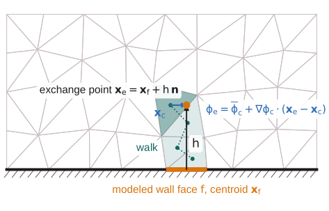
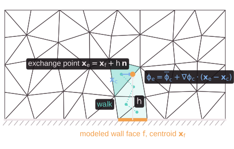
Location. At setup, each point is located by a walk through the local mesh: from the wall cell, the walk crosses the face of the current cell beyond which the point lies farthest, the largest \((\mathbf{x}_e - \mathbf{x}_{f'})\cdot\mathbf{n}_{f'}^\mathrm{out}\) over its faces \(f'\), until the point is inside the cell to a tolerance of \(10^{-10}\) (double precision; \(10^{-5}\) in single) times the cell size. Crossing a periodic seam shifts the point into the frame of the cell entered. A walk that leaves the domain (a point beyond the opposite wall, past a concave corner, or across a thin region) is an input error naming the face; one that reaches the edge of the halo deepens it (below). The containing cell \(c\) and the offset \(\mathbf{x}_e - \mathbf{x}_c\) are stored per face.

Sampling. At every stage, the primitive state \(\mathbf{W} = [\rho, \mathbf{u}, p]\) at the point is reconstructed linearly in the containing cell from its cell average and its gradient for the viscous terms (chapter 6):

\[ \begin{equation} \mathbf{W}_e = \overline{\mathbf{W}}_c + \nabla\mathbf{W}_c\cdot(\mathbf{x}_e - \mathbf{x}_c), \qquad T_e = \frac{p_e}{\rho_e R}, \label{eq:sampling} \end{equation} \]

exact for linear fields on every cell type; if the reconstruction gives a non-positive density or pressure, the cell average is used instead. The model's inputs are the speed relative to the wall in the plane of the face,

\[ \begin{equation} \mathbf{u}_\parallel = (\mathbf{I} - \mathbf{n}\mathbf{n})(\mathbf{u}_e - \mathbf{u}_w), \qquad U_m = \lvert\mathbf{u}_\parallel\rvert, \label{eq:tangential-velocity} \end{equation} \]

with \(\mathbf{u}_w\) the wall's velocity, the temperature \(T_m = T_e\) and the pressure \(p = p_e\), which the models hold constant across the layer, so that \(\rho = p/(RT)\) there.

Equilibrium ODE model

model = "equilibrium" (Kawai & Larsson 2012; Larsson et al. 2016) solves the thin-layer momentum and energy equations along the wall-normal coordinate \(y \in [0, h]\):

\[ \begin{align} \frac{\mathrm{d}}{\mathrm{d}y}\left[(\mu + \mu_t)\frac{\mathrm{d}u}{\mathrm{d}y}\right] &= 0, \label{eq:ode-momentum} \\ \frac{\mathrm{d}}{\mathrm{d}y}\left[(\mu + \mu_t)\,u\frac{\mathrm{d}u}{\mathrm{d}y} + c_p\left(\frac{\mu}{Pr} + \frac{\mu_t}{Pr_t}\right)\frac{\mathrm{d}T}{\mathrm{d}y}\right] &= 0, \label{eq:ode-energy} \end{align} \]

with the gas's \(\mu(T)\), \(c_p\) and \(Pr\), and a mixing-length eddy viscosity with van Driest damping (van Driest 1956) in semi-local units:

\[ \begin{equation} \mu_t = \kappa\,y\sqrt{\rho\,\tau_w}\,D(y^*), \qquad D(y^*) = \left[1 - \exp(-y^*/A^+)\right]^2, \qquad y^* = \frac{y\sqrt{\rho\,\tau_w}}{\mu}, \label{eq:mixing-length} \end{equation} \]

\(\kappa\) = kappa (0.41), \(A^+\) = A_plus (17) and \(Pr_t\) = Pr_t (0.9), with \(\rho\) and \(\mu\) the local values. The boundary conditions are \(u = 0\) at the wall and \(u = U_m\), \(T = T_m\) at \(y = h\), with \(T = T_w\) at an isothermal wall and \(-k\,\mathrm{d}T/\mathrm{d}y = q\) at a heat-flux wall (adiabatic: \(q = 0\)). Both equations state that a flux is constant across the layer,

\[ \begin{equation} (\mu + \mu_t)\frac{\mathrm{d}u}{\mathrm{d}y} = \tau_w, \qquad k_\mathrm{eff}\frac{\mathrm{d}T}{\mathrm{d}y} + \tau_w u = -q_w, \qquad k_\mathrm{eff} = c_p\left(\frac{\mu}{Pr} + \frac{\mu_t}{Pr_t}\right), \label{eq:constant-fluxes} \end{equation} \]

so for given \(\mu_t\) and properties the profiles follow by quadrature, and the boundary values fix the wall fluxes. With \(I_1 = \int_0^h \mathrm{d}y/(\mu + \mu_t)\), \(I_2 = \int_0^h \mathrm{d}y/k_\mathrm{eff}\) and \(I_3 = \int_0^h u\,\mathrm{d}y/k_\mathrm{eff}\),

\[ \begin{equation} \tau_w = \frac{U_m}{I_1}, \qquad q_w = \frac{T_w - T_m - \tau_w I_3}{I_2} \quad \text{(isothermal)}, \qquad T_w = T_m + q I_2 + \tau_w I_3 \quad \text{(heat flux)}. \label{eq:ode-solution} \end{equation} \]

At a heat-flux wall \(q_w = q\) and the model returns the wall temperature. In the laminar limit (\(\mu_t \to 0\), constant properties) these reduce to Couette flow, \(\tau_w = \mu U_m/h\) and \(q_w = -[k(T_m - T_w) + \mu U_m^2/2]/h\).

Solver. The layer is discretized by \(N = 64\) nodes stretched geometrically toward the wall,

\[ \begin{equation} y_j = h\,\frac{r^j - 1}{r^{N-1} - 1}, \qquad j = 0, \dots, N - 1, \qquad r = 1.1, \label{eq:wall-model-grid} \end{equation} \]

whose first spacing, \(2.5\times10^{-4}\,h\), keeps \(y_1^+ < 1\) up to \(h^+ \approx 4000\). The integrals are evaluated by Simpson's rule on each interval, with the values at its midpoint. The profiles start linear between the wall and the exchange point (at a heat-flux wall from \(T_m\)), and \(\tau_w\) from the larger of the laminar stress \(\mu_w U_m/h\) and the log law \(U_m/u_\tau = \kappa^{-1}\ln(h u_\tau/\nu_w) + 5.2\) at the wall's properties. Each iteration evaluates \(\mu_t\) and the properties on the current profiles, then \(\tau_w\), \(q_w\) (or \(T_w\)) and new profiles from eqs. \(\eqref{eq:constant-fluxes}\)-\(\eqref{eq:ode-solution}\). The fixed point is accelerated by secant steps on the residual of \(\tau_w\) (accepted when they stay within a factor of 2 of the plain update) and ends when \(\tau_w\) changes by at most \(10^{-10}\) relatively and the temperature at every node by at most \(10^{-10}\), or after 200 iterations. At constant properties it takes 4-5 iterations from \(h^+ = 5\) to \(7000\); with strong heating (\(T_m/T_w = 1.6\) at a Mach number of 0.7, \(\mu \propto T^{0.75}\)) 8-20.

Griffin-Fu-Moin model

model = "gfm", the default (Griffin, Fu & Moin 2023), builds the compressible velocity profile by inverting the velocity transformation of Griffin, Fu & Moin (2021), which maps compressible profiles with and without heat transfer onto the incompressible law of the wall. With \(U^+ = U/u_\tau\), \(\mu^+ = \mu/\mu_w\) and \(\rho^+ = \rho/\rho_w\), the transformation is

\[ \begin{equation} S_t^+ = \frac{S_\mathrm{eq}^+}{1 + S_\mathrm{eq}^+ - S_\mathrm{TL}^+}, \qquad S_\mathrm{eq}^+ = \frac{1}{\mu^+}\frac{\mathrm{d}U^+}{\mathrm{d}y^*}, \qquad S_\mathrm{TL}^+ = \mu^+\frac{\mathrm{d}U^+}{\mathrm{d}y^+}, \label{eq:gfm-transformation} \end{equation} \]

and the incompressible law it is inverted against is the constant-property version of the mixing length \(\eqref{eq:mixing-length}\),

\[ \begin{equation} S_t^+ = \frac{1}{1 + \kappa\,y^* D(y^*)}. \label{eq:incompressible-law} \end{equation} \]

Solving \(\eqref{eq:gfm-transformation}\) for the velocity gradient, with \(y^* = y^+\sqrt{\rho^+}/\mu^+\), gives the profile from the wall outward:

\[ \begin{equation} \frac{\mathrm{d}U^+}{\mathrm{d}y^*} = \left[\frac{1}{\mu^+ S_t^+} - \frac{1}{\mu^+} + \sqrt{\rho^+}\left(1 + \frac{y^+}{2\rho^+}\frac{\mathrm{d}\rho^+}{\mathrm{d}y^+} - \frac{y^+}{\mu^+}\frac{\mathrm{d}\mu^+}{\mathrm{d}y^+}\right)\right]^{-1}. \label{eq:gfm-inverse} \end{equation} \]

The temperature, hence \(\rho^+\) and \(\mu^+\), follows the velocity by the generalized Reynolds analogy of Zhang et al. (2014), with its quadratic coefficient set so that the relation passes through the exchange point \((U_m, T_m)\):

\[ \begin{align} T(U) &= T_w + s\,Pr\,(T_r - T_w)\frac{U}{U_e}\left(1 - \frac{U}{U_m}\right) + \left(\frac{U}{U_m}\right)^2(T_m - T_w), \label{eq:reynolds-analogy} \\ T_r &= T_e + Pr^{1/3}\frac{U_e^2}{2c_p}, \label{eq:recovery-temperature} \end{align} \]

with \(s\) = s (1.14), the recovery temperature \(T_r\) of recovery factor \(Pr^{1/3}\), and the edge speed and temperature \(U_e\), \(T_e\). The wall heat flux is that of this relation at the wall, \(q_w = -k_w (\mathrm{d}T/\mathrm{d}U)_w (\mathrm{d}U/\mathrm{d}y)_w\):

\[ \begin{equation} q_w = \frac{s\,\tau_w c_p (T_w - T_r)}{U_e}. \label{eq:gfm-heat-flux} \end{equation} \]

An adiabatic wall takes \(T_w = T_r\), so \(q_w = 0\); an isothermal wall its temperature. Walls with a prescribed non-zero heat flux are rejected (use the equilibrium model). Without shear (\(U_m = 0\)) the model returns \(\tau_w = 0\) and the conduction flux \(q_w = -c_p\mu_w(T_m - T_w)/(Pr\,h)\).

Solver. On the grid \(\eqref{eq:wall-model-grid}\), each interval applies \(\eqref{eq:gfm-transformation}\) in difference form, with \(\mu^+\) the mean of its two nodes and \(S_t^+\) averaged over the interval in \(y^*\) by Simpson's rule; solving for the increment,

\[ \begin{equation} \Delta U^+ = \frac{S_t^+}{(1 - S_t^+)/(\mu^+\Delta y^*) + S_t^+\mu^+/\Delta y^+}. \label{eq:gfm-increment} \end{equation} \]

The differences of \(y^*\) carry the density and viscosity derivatives of \(\eqref{eq:gfm-inverse}\), and with constant properties \(\Delta U^+ = S_t^+\Delta y^+\). Because \(y^*\) at the upper node depends on its temperature, hence on its velocity, each interval predicts the velocity from the previous increment and corrects it three times. The profile's \(U(h)\) increases with \(\tau_w\), and \(\ln U(h)\) is nearly linear in \(\ln\tau_w\): \(\tau_w\) is found by secant steps on \(\ln\tau_w\) for the root of \(\ln[U(h)/U_m]\), from the initial estimate of the equilibrium model, with steps limited to a factor \(e^2\), to \(10^{-9}\) in \(\ln\tau_w\). It takes 4-7 profile evaluations from \(h^+ = 5\) to \(7000\), with or without heat transfer.

Edge state

The Reynolds analogy needs the speed and temperature at the boundary-layer edge (in a channel, at the centerline). They are sampled like the exchange point \(\eqref{eq:sampling}\) at the edge point, a distance edge_distance along the normal: the half-height of a channel or pipe, an estimate of \(\delta\) in a boundary layer. \(U_e\) is the tangential speed relative to the wall there, bounded below by \(U_m\).

Coupling to the LES

On a modeled wall face the model's output replaces the viscous flux. The fluid receives the traction and heat flux

\[ \begin{equation} \mathbf{t}_w = -\tau_w\frac{\mathbf{u}_\parallel}{U_m}, \qquad \dot{E}_w = q_w + \mathbf{u}_w\cdot\mathbf{t}_w, \label{eq:wall-flux} \end{equation} \]

per unit area of the face, opposite to the velocity relative to the wall and including the work of a moving wall; there is no normal viscous stress and no SGS flux on the face (ViscousFluxFunctor::modeled_flux, src/numerics/viscous_flux.h). The exterior state of the face is that of a slip wall (chapter 9): the normal velocity mirrored, the tangential velocity, density and pressure of the interior. The convective flux therefore carries the pressure force only, and the reconstruction, the gradients and the eddy viscosity of the wall cells see no velocity jump to the wall: with the no-slip exterior state the wall cell's gradient would hold the jump from the wall to a first cell in the log layer, a shear the LES does not resolve. The wall temperature of an isothermal modeled wall enters only through the model.

The models are evaluated at every stage of the time integration, after the gradients of the viscous terms and the eddy viscosity, by one kernel over the modeled wall faces of the owned cells. Their inputs are instantaneous, not time-filtered. [[forces]] monitors of modeled zones report the modeled traction and add the integrated heat flux into the fluid (Probes and monitors).

Parallel runs and restarts

The wall flux of a face depends on the state and gradients of the cells containing its exchange and edge points, which may belong to another rank. Rather than sending these values during the time loop, the halo is made deep enough that both cells are local with complete gradient stencils: a point found in halo layer \(L\) needs \(L + 1\) layers (the outermost layer's gradients miss neighbors), and a walk that reaches the edge of the halo needs one more layer than the current depth. The deepest requirement over all ranks sets the halo depth, and the setup after the mesh is repeated, as for TENO-E stencils (MPI design notes); when the halo is then trimmed, the containing cells and their vertex neighbors are kept. The wall flux is therefore computed from the same values on any number of ranks, and the results are independent of the partition. The cost is a deeper halo where a partition boundary runs parallel to a wall within \(h\) (or edge_distance) of it.

The models keep no state between stages, so restart files carry nothing new and a restarted run reproduces an uninterrupted one bitwise.

Limitations

• Single gases only; gas mixtures are rejected (they will follow isothermal mixture walls). Axisymmetric runs are not supported. [physics] must be navier_stokes.
• Equilibrium models only: no pressure-gradient or convective terms in the layer, so no model of non-equilibrium boundary layers (strong pressure gradients, separation) yet.
• The Griffin-Fu-Moin model supports isothermal and adiabatic walls, and takes the edge state at a fixed distance rather than detecting the boundary-layer edge.
• The modeled wall flux and the force monitors include no SGS contribution at the wall.

The validation against the channels of Lee & Moser (2015) and Trettel & Larsson (2016) is in the design notes.